Bayesian Analysis for Epidemiologists II: Markov Chain Monte Carlo

Acknowledgements

I am indebted to the following individuals upon who’s work the material in these pages has been (extensively) based. For the material on grid sampling, I leaned particularly heavily on material presented by Shane Jensen as part of a Statistical Horizons course. If you want to pursue this in any real way, you should very much attend that course.

Jim Albert
David Spiegelhalter
Nicky Best
Andrew Gelman
Bendix Carstensen
Lyle Guerrin
Shane Jensen and Statistical Horizons

Sections

I. Grid Sampling
1. The Multi-Parameter Normal Model
2. Random Sampling From a Standard Distribution
3. Grid Sampling From a Non-Standard Distribution
4. Grid Sampling for Airline Crash Example

II. MCMC
1. Introduction to Monte Carlo
2. Introduction to Markov Chain Monte Carlo
3. The Metropolis Algorithm
4. Gibbs Sampling
5. Running MCMC in BUGS

Grid Sampling

In the first part of this discussion, we considered relatively simple one-parameter models and conjugate analysis. Before we move on to the kinds of Markov Chain Monte Carlo methods in common use for more complex problems, we’ll take some first steps toward realistic problems that require computational methods. The first such method is called grid sampling, which we present in the setting of both normal and Poisson models.

The Multi-Parameter Normal Model

In our introduction to the single-parameter normal model, we assumed (somewhat unrealistically) that we didn’t know the mean, but somehow did know the variance. We now take the more real-world stance that both the mean and the variance are unknown. So now, \(\sigma^2\) doesn’t drop out of the model specification, making the Bayesian calculations more complicated. You may begin to appreciate that even for this relatively simple model, the simple analytic approaches we’ve seen in the previous conjugate analyses become increasingly more difficult to apply, and we begin to see the need for computational approaches.¹

The maximum likelihood estimates for both parameters are fairly straightforward: \(\mu_{MLE} = \bar{y}\) and \(\sigma^2_{MLE} = \Sigma(y-\bar{y})^2/n\). But, for a Bayesian approach to the normal likelihood (\(y_i \sim Normal(\mu, \sigma^2)\)), we’ll need conjugate priors for both parameters. This complicates matters somewhat. A fully conjugate prior for the mean (\(\mu|\sigma^2 \sim Nl(\mu_0, \sigma^2/\kappa_0)\)) and the standard deviation (\(\sigma^2 \sim Inverse Gamma (...)\) ²) will require us to look at the joint distribution of the two parameters simultaneously. Even in this relatively simple setting, this is not necessarily a simple thing to do, and it only gets more complex when we start to consider semi-conjugate and non-informative priors.

As a first approach, we can break the joint distribution for the mean and standard deviation into two easier components. Start with the marginal posterior distribution for \(\sigma^2\), \(p(\sigma^2|y)\), then move to the conditional posterior for \(\mu\), \(p(\mu|\sigma^2, y)\). The difficult bit is \(p(\sigma^2|y)\), the formula for which is appropriately gnarly:

But when we have the prior distribution for \(\sigma_{2}\), it becomes a one-parameter problem, with the notable caveat that in this fully conjugate specification, \(\mu\) is dependent on \(\sigma^2\).

Random Sampling From a Standard Distribution

We are often interested in a minimally or non-informative prior. In the setting of a multi-parameter normal model this would be: \(p(\sigma^2|y) \sim InvGamma(n/2, \Sigma(y-\bar{y})^2/2)\). The approach is to first sample from \(p(\sigma^2|y)\), then plug those values into a simulation for \(\mu\). To sample from the inverse Gamma, we sample from the Gamma, then inverse it.

In the following code, we first load and plot data for 60 observations of average yearly temperatures in New Haven, Connecticut in the US. We then loop through the two-step sampling scheme for \(\mu\) and \(\sigma^2\) and then compare the raw data to the posterior sample using a histogram.³

1
2
3
4
5
6
7
8
9
10
11
12
13
14
15
16
17
18
19
20
21
22
23
24
25
26
27
28
29
30
31
32
33
34
35
36
37
38
39
40
41
42

  ### Observed Data: Average Yearly Temperatures in New Haven over 60 years

  data(nhtemp)
  y <- nhtemp

  ### Plotting Observed Data

  par(mfrow=c(1,1))
  hist(y,col="gray")

  ### Summary Statistics

  n <- length(y)
  y.bar <- mean(y)
  y.ss <- sum((y-y.bar)^2)

  # (run through the 2-step sampling scheme)
  ### Posterior Samples of mu and sigma^2 with non-informative prior

  mu.samp <- rep(NA,10000) # vectors to store values
  sigsq.samp <- rep(NA,10000)
  for (i in 1:10000){
     x <- rgamma(1,shape=n/2,rate=y.ss/2)
     sigsq.samp[i] <- 1/x # inverse the gamma
     mu.var <- sigsq.samp[i]/n
     mu.mean <- y.bar    
     mu.samp[i] <- rnorm(1,mean=mu.mean,sd=sqrt(mu.var))
 # (use value of sigma.sq to sample for mu)
  }

  ### Plotting Posterior Samples of mu and sigmasq

  par(mfrow=c(2,1))
  hist(sigsq.samp,col="gray",main="Posterior Distribution of Sigsq")
  hist(mu.samp,col="gray",main="Posterior Distribution of mu")

  ### Comparing Posterior Samples of mu to raw data

  mintemp <- min(y)
  maxtemp <- max(y)
  par(mfrow=c(2,1))
  hist(y,col="gray",main="Distribution of Data",xlim=c(mintemp,maxtemp))
  hist(mu.samp,col="gray",main="Posterior Distribution of mu",xlim=c(mintemp,maxtemp))

Grid Sampling From a Non-Standard Distribution

For a more reasonable approach to a normally distributed variables, we will want to remove the dependency between \(\mu\) and \(\sigma^2\). A semi-conjugate prior will help us accomplish this, but will complicate the algebra enough to push us to computational approaches. Up to now, we could get at \(p(\sigma^2|y)\) through an Inverse Gamma, which as we’ve seen is intimidating looking, but still standard. To remove the dependency between \(\mu\) and \(\sigma^2\) we will have to sample from a non-standard distribution:

Grid sampling is a way to sample from any non-standard distribution, which opens up the possibilities for more realistic, more complicated analyses.⁴

In grid sampling we plug a series of values into a formula, such as the the formula for the non-standard posterior for \(\sigma^2\) above, get back probabilities for each of those values, and then sample those values over and over again relative to those probabilities. The difficult bit is coming up with a grid of values to plug into the formula that adequately and reasonably explores the posterior probability space.⁵ There is something of an art to finding a good grid of values that adequately explores the posterior distribution space. Grid sampling generally involves a manual approach to selecting candidate values. There are, though, automated schemes to search the sample space, which we will talk about soon.

Let’s apply the grid sampling approach with a semi-conjugate prior to the yearly temperature example. After reading in and plotting the raw data and setting a couple of statistics, we define values for the hyperparameters. Next, we write the function to enter values into the formula for the non-standard posterior distribution for \(\sigma^2\). After that, we use the pppoints() function to create a grid of 100 points between 0 and 6. This step is not trivial. Determining the limits of 0 and 6 in this example is is the result of a tedious and time consuming ⁶ process of trial and error explorations and iterations to arrive at values that optimally explore the probability space.

At this point we have a grid of values and relative probabilities for \(\sigma^2\). The next step is to draw 1,000 samples for \(\sigma^2\) proportional to those probabilities. This establishes the posterior distribution of \(\sigma^2\), which we then use to sample the second parameter in the normal distribution, \(\mu\), and finally arrive at the posterior distribution for \(\mu\) itself.

1
2
3
4
5
6
7
8
9
10
11
12
13
14
15
16
17
18
19
20
21
22
23
24
25
26
27
28
29
30
31
32
33
34
35
36
37
38
39
40
41
42
43
44
45
46
47
48
49
50
51
52
53
54
55
56
57
58
59
60
61
62
63
64
65
66
67
68
69
70
71
72
73
74
75
76
77
78
79
80
81

 ### Data: Average Yearly Temperatures in New Haven over 60 years

data(nhtemp)
y <- nhtemp

 ### Plot Observed Data

par(mfrow=c(1,1))
hist(y,col="gray")

 ### set up some stats

n <- length(y)
y.bar <- mean(y)
y.ss <- sum((y-y.bar)^2)

 ## set hyperparameter values for prior 

tausq0 <- 5
sigsq0 <- 5
nu0 <- 1
mu0 <- 50

 ## write function to evaluate posterior distribution of sigsq over a grid
 # (this is that gnarly function into which we plug in the grid of values)
 
evaluatepostsigsq <- function(sigsqgrid,y,mu0,nu0,tausq0,sigsq0){
    logvals <- rep(0,length(sigsqgrid))
    for (i in 1:length(sigsqgrid)){
        cursigsq <- sigsqgrid[i]
        postmean  <- (n*y.bar/cursigsq + mu0/tausq0)/(n/cursigsq + 1/tausq0)
        for (j in 1:n){
            logvals[i] <- logvals[i] + dnorm(y[j],mean=postmean,sd=sqrt(cursigsq))
        }
        logvals[i] <- logvals[i] - 0.5*log(n/cursigsq + 1/tausq0)
        logvals[i] <- logvals[i] - (0.5*nu0+1)*log(cursigsq) - nu0*sigsq0/cursigsq
        print (i)
    }
    out <- exp(logvals-max(logvals))
    out
}

 # create grid of values to plug into the function (the tough part...)


sigsqgrid <- ppoints(100)*6  ## grid of 100 points between 0 and 6

 # feed the grid of probabilities to the function for the formula
sigsqprobs <- evaluatepostsigsq(sigsqgrid,y,mu0,nu0,tausq0,sigsq0)
par(mfrow=c(1,1))
plot(sigsqgrid,sigsqprobs,type="l",main="Posterior Dist. of Sigsq (Semi-Conjugate Prior)")


 ## grid sampling: sample 1000 values sigsq proportional to sigsqprobs

sigsqprobs <- sigsqprobs/sum(sigsqprobs)
sigsq.samp <- sample(sigsqgrid,size=1000,replace=T,prob=sigsqprobs) 
# (use sample() to do multinomial sample from whole vector of probabilities)

 ## plot posterior distribution sigsq

par(mfrow=c(2,1))
plot(sigsqgrid,sigsqprobs,type="l",main="Posterior Dist. of Sigsq (Semi-Conjugate Prior)")
hist(sigsq.samp,prob=T,main="Posterior Samples of Sigsq (Semi-Conjugate Prior)",col="gray")


 ## sample mu, given sampled sigmasq, 

mu.samp.semiconjugate <- rep(NA,1000) # create vector to store samples
for (i in 1:1000){
    mu.var <- 1/(n/sigsq.samp[i] + 1/tausq0)
    mu.mean <- (n*y.bar/sigsq.samp[i] + mu0/tausq0)*mu.var
    mu.samp.semiconjugate[i] <- rnorm(1,mean=mu.mean,sd=sqrt(mu.var))
}

 ### compare posterior samples of mu to raw data

mintemp <- min(y)
maxtemp <- max(y)
par(mfrow=c(2,1))
hist(y,col="gray",main="Distribution of Data",xlim=c(mintemp,maxtemp))
hist(mu.samp.semiconjugate,col="gray",main="Posterior
 Distribution of mu (Semi-Conjugate Prior)",xlim=c(mintemp,maxtemp))

The benefits of grid sampling are that it is conceptually straightforward and can be used to evaluation most any function of values. The disadvantages are that it requires quite a bit of work to manually tune the sampler.

Grid Sampling for Airline Crash Example

In the section on simple conjugate analyses there was an example of a Poisson model for airline crash data that assumed the same underlying rate for all 10 annual realizations of the Poisson processes: \(y \sim Poisson(\theta)\). The prior for \(\theta\) was a minimally informative \(Gamma(\alpha=0, \beta=0)\). The posterior was the closed standard distribution \(\theta|y \sim Gamma(\Sigma y_i + \alpha, n + \beta)\).

When we plot the data, though, it appears crashes were decreasing over time. A more realistic and valid model would account for that time trend. The simplest approach would be to model the trend linearly: \(y \sim Poisson(\alpha + \beta * t)\). But simply plugging \((\alpha + \beta * t)\) into the Poisson likelihood, results in a complicated function for which there is no easy derivative. We will have to specify a prior for both \(\alpha\) and \(\beta\), which results in non-standard distributions for \(\alpha\) and \(\beta\).

This is more complex than the previous normal distribution example. We now have to sample for 2 unknown variables (\(\alpha\) and \(\beta\)). One approach utilizes a 2-dimensional grid of values, from which samples are drawn to simulate the target distributions. The grid will be quite large. For example, to obtain 100 samples for each of the two parameters, we will need \(100^2\) or 10,000 different values. As before, we then have to plug those (10,000) values into the target function and calculate probabilities.

Operationally, it’s more efficient to break the problem down into 2 steps: first, sample from \(\alpha\), then sample \(\beta |\alpha\). Rather than directly evaluating the joint probability distribution of 10,000 values, we can sample from 100 values of \(\alpha\) then sample \(\beta\) given \(\alpha\). Think of it in terms of a contingency table. The \(\beta\) values are arrayed along the x-axis (columns) and \(\alpha\) values along y-axis (rows). The \(\alpha\) values are a marginal distribution, or the sum of the \(\beta\)’s for that value (row) of alpha. The following code is from Dr. Shane Jensen’s course on applied Bayesian data analysis⁷, and illustrates grid sampling for the airline crash data.

After setting up the data and looking at a quick plot, write the formula for the posterior as a function. Again, the ppoints() R function returns equally spaced points that we will use to populate the formula for the posterior. And again, the choice of the limits for the grid sampler (between 20 and 40 for alpha and between -3 and 3 for beta) is the result of painstaking trial and error on Dr. Jensen’s part. After defining the grid, plug the values into the formula for the posterior, and use the countour() function to illustrate the probability space. After that, calculate the probabilities for the grid sampler values. First look at the marginal distribution of alpha, then look at beta conditional on alpha. Plot the marginal distribution for alpha, and the conditional distribution for beta. After that, we get to the business of sampling alpha and beta values conditional on their probabilities from the grid sampling and plotting the results. Finally, characterize and plot the posterior predictive distribution for these data using our results.

1
2
3
4
5
6
7
8
9
10
11
12
13
14
15
16
17
18
19
20
21
22
23
24
25
26
27
28
29
30
31
32
33
34
35
36
37
38
39
40
41
42
43
44
45
46
47
48
49
50
51
52
53
54
55
56
57
58
59
60
61
62
63
64
65
66
67
68
69
70
71
72
73
74
75
76
77
78
79
80
81
82
83
84
85
86
87
88
89
90
91
92
93
94
95
96
97
98
99
100
101
102

 # fatal airline crashes over 10 years

 years <- c(1976,1977,1978,1979,1980,1981,1982,1983,1984,1985)
 crashes <- c(24,25,31,31,22,21,26,20,16,22)
 years <- years-1976
 n <- length(years)

 # plot trend over time

 par(mfrow=c(1,1))
 plot(years,crashes,pch=19)

 numgrid <- 100

 # formula to evaluate posterior over range of alpha and beta:

 posteriorplanes <- function(alpha,beta){
   logpost <- -Inf
   if (alpha + beta*max(years) > 0){
     logpost <- 0
     for (i in 1:n){
       logpost <- logpost + crashes[i]*log(alpha+beta*years[i])
       logpost <- logpost - (alpha+beta*years[i])
     }
   }
   logpost
 }
   
  # set up grid sampler
 alpharange <- ppoints(numgrid)*20+20   # alpha between 20 and 40 
 betarange <- ppoints(numgrid)*6-3  # beta between -3 and 3
 full <- matrix(NA,nrow=numgrid,ncol=numgrid)
 for (i in 1:numgrid){
   for (j in 1:numgrid){
     full[i,j] <- posteriorplanes(alpharange[i],betarange[j])
   }
 }
 full <- exp(full - max(full))
 full <- full/sum(full)
 contour(alpharange,betarange,full,xlab="alpha",ylab="beta",drawlabels=F)

 ## calculate probabilities for grid sampler  (alpha first, then beta conditional on alpha)
 alphamarginal <- rep(NA,numgrid)
 for (i in 1:numgrid){
   alphamarginal[i] <- sum(full[i,])
 }
 betaconditional <- matrix(NA,nrow=numgrid,ncol=numgrid)
 for (i in 1:numgrid){
   for (j in 1:numgrid){
     betaconditional[i,j] <- full[i,j]/sum(full[i,])
   }
 }

 ## plot marginal distribution of alpha
 par(mfrow=c(1,1))
 plot(alpharange,alphamarginal,type="l",main="marginal dist. of alpha")

 ## plot conditional distribution of beta
 par(mfrow=c(3,1))
 plot(betarange,betaconditional[25,],type="l",main="dist. of beta for alpha = 24.9")
 plot(betarange,betaconditional[50,],type="l",main="dist. of beta for alpha = 29.9")
 plot(betarange,betaconditional[75,],type="l",main="dist. of beta for alpha = 34.9")

 ## sample grid values:
 alpha.samp <- rep(NA,10000)
 beta.samp <- rep(NA,10000)
 for (m in 1:10000){
   a <- sample(1:100,size=1,replace=F,prob=alphamarginal)
   b <- sample(1:100,size=1,replace=F,prob=betaconditional[a,])
   alpha.samp[m] <- alpharange[a]
   beta.samp[m] <- betarange[b]
 }

 par(mfrow=c(1,1))
 contour(alpharange,betarange,full,xlab="alpha",ylab="beta",drawlabels=F,col=2)
 points(alpha.samp,beta.samp)

 ## plot posterior samples for alpha and beta
 par(mfrow=c(2,1))
 hist(alpha.samp,main="Alpha Samples",col="gray")
 hist(beta.samp,main="Beta Samples",col="gray")


 par(mfrow=c(1,1))
 plot(years,crashes,pch=19)
 for (i in 1:500){
   abline(alpha.samp[i],beta.samp[i],col=3)
 }
 points(years,crashes,pch=19)

 ## plot post pred distn for crashes for 1986 (years = 10)

 pred.rate <- alpha.samp + beta.samp*10

 pred.crashes <- rep(NA,10000)
 for (i in 1:10000){
   pred.crashes[i] <- rpois(1,pred.rate[i])
 }

 par(mfrow=c(2,1))
 hist(crashes,xlim=c(0,45),main="Observed Data 1976-1985",col="gray",breaks=10)
 hist(pred.crashes,xlim=c(0,45),main="Posterior Predictive for 1986",col="gray")

In the plot of the possible annual trend line, notice that some of the possible slope lines show an increase in the annual trend of airline crashes. There are few of those lines, so such an increase is unlikely. But it is possible, and this might not be immediately apparent in standard statistical approaches. We can quantify the probability of a decreasing trend over time by calculating the proportion of posterior probability for \(\beta\) that is less than zero. In this example it is 96%. So the probability that the trend is actually increasing is 4%. This is a direct probability statement. Also notice that allowing the intercept to vary affects the slope. Larger values for the intercept invariably force more negative slopes to fit the data to the points. This correlation between slope and intercept is also not immediately apparent in classical regression. Because the grid approach is finite, we will also see artifactual white spaces in the plots.

MCMC

Up until the late 1980s, Bayesian inference consisted primarily of conjugate models. While the prior and the likelihood could usually be described in closed form, for most reasonably realistic models, the posterior was often not analytically tractable. The introduction of theory and computing power to employ Monte Carlo methods led to a way to get at more complex problems, and has resulted in something of a revolution in Bayesian statistics. Not only can Monte Carlo can be used to simulate values from closed forms of prior and posterior distributions, it is the basis for Markov Chain algorithms to sample from arbitrary (typically high-dimensional) posterior distributions that would otherwise not be amenable to analysis. These Monte Carlo samples allow approximations to the integral of otherwise intractable distributions. The basic concepts of sampling and simulation are the same as simple Monte Carlo, but we sample from non-closed form distributions. Theorems exist which prove convergence to the integral as the sample size approaches infinity, even if the sampling is not independent. Monte Carlo algorithms form the approach of much of modern Bayesian analysis.

A Markov chain describes a series of possible events where the probability of the next event depends solely on the current place. The term Monte Carlo arose during WWII, when folks like Stanislaw Ulam and Nicholas Metropolis were working on the Manhattan Project, and refers to estimating statistical models with sampling. A major challenge in estimating complex (multi-dimensional) posterior distributions is coming up with a good range of possible values to explore. Algorithms like expectation-maximization (EM) algorithm are pretty good at arriving at point estimates, but not very good at fully describing a probability space. Think of a posterior distribution as a series of peaks and valleys of probabilities. When we are interested in evaluating samples from that distribution, rather than march straight up the hill to the most likely value by the quickest route possible, we are better off meandering around a bit and exploring the terrain before eventually ascending to the peak. One of the most popular approaches to conducting this exploration is the Gibbs sampler, which is named after the 19th-century American scientist J. Willard Gibbs, who contributed to the invention of statistical mechanics and vector calculus.

Introduction to Monte Carlo

BUGS programs (of which WinBUGS, OpenBUGS and JAGS are the most popular) use a Monte Carlo approach to estimating probabilities, summary statistics and tail areas of probability distributions. Monte Carlo itself, is basically simulation. Say you are interested in the probability of 8 or more heads in 10 tosses of a fair coin. We could use the binomial formula to get an exact answer (it is 0.0547). Or you could take a physical approach and toss 10 coins repeatedly into the air, and count up how many times out of how many tosses we get 8 or more heads. Simulation uses a computer to “toss the coins”. Here is some R code that does just that:

1
2

coins<-rbinom(10000,10,.5)
length(coin[coin>7])/length(coin)

Ten thousand simulations gets close to the exact answer. And a computer will not complain if you ask for a hundred thousand tosses. This is the basis of Monte Carlo approaches: simulate by sampling from some distribution and summarize the results as a probability distribution. You can also calculate a so-called Monte Carlo error on your results, which is the \(\frac{\sigma^2_{sample}}{\sqrt{n_{iterations}}}\) The MC error decreases with the number of iterations, and can be used as an estimate of how close your estimate is to an exact estimate.

Monte Carlo Calculation of Pi

Let’s look at another simple simulation example. ⁸ Imagine you are throwing darts, but for reasons know only to folks who make up probability examples, you are just interested in hitting the dartboard in the upper right corner. at the following figure.

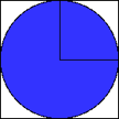
Dart Board 1

Dart Board 2

Further imagine (for the same obscure reasons) you are a very, very poor dart player. In fact your darts are essentially random tosses. If you throw enough darts, eventually, the number of darts that hit the upper right corner will be proportional to that area. The ratio of the number of darts that hit the shaded area to the total number of darts thrown will, in fact, equal one-fourth the value of pi.

We can create a “virtual” dart board by generating x and y coordinates values, and calculate the distance from the origin (0,0) using the Pythagorean theorem. If the circle’s radius is 1, then values that are less than 1 fall in the shaded area, and values that are more than one fall outside the area. Do this enough times, and we can get a reasonable approximation of pi.

Here’s some R code that accomplishes that.

1
2
3
4
5
6

x<-runif(1000)
y<-runif(1000,)
distance<-sqrt(x^2+y^2)
hits<-distance[distance<1]
quart.pi<-length(hits)/length(distance)
4*quart.pi

Run this code and I think you will find that just 1,000 “throws” gets us pretty close. This, then, is the essence of a Monte Carlo simulation.

Introduction to Markov Chain Monte Carlo

While we may be able to get a lot of mileage out of the simple conjugate analyses we considered in the first section (and, in fact even the most sophisticated modern software will resort to conjugacy if it applies), we will very likely run out of gas when we try to address more realistic and complex problems. There are a couple of options for when we have a likelihood function and prior distribution that can’t be handled by formal, mathematical (read conjugate) analysis. We could take a so-called “grid” approach by specify a prior with a dense grid of say 1,000 values spanning all possible values of \(\theta\). This may be reasonable when dealing with one parameter, but imagine the case of 6 parameters. We would need \(1000^6\) combinations of values. That’s (1,000,000,000,000,000,000 for those of you keeping score.)

Many of the limitations on the use of Bayesian statistics were solved when theoretical and computing advances allowed the use of sampling algorithms that produce a large number of representative values of most any posterior distribution of \(\theta\). We can then calculate things like means and variances using those representative values. Independent sampling from a joint posterior distribution like \(p(\theta | y)\) is difficult, but dependent sampling from a Markov Chain, where each value is conditional on the previous value, is easier. There are several standard ‘recipes’ available for designing Markov chains for a stationary target distribution. The basic version is the Metropolis algorithm (Metropolis et al, 1953), which was generalized by Hastings (1970). Gibbs Sampling is a special case of the Metropolis-Hastings algorithm which generates a Markov chain by sampling from the full set of conditional distributions. Hopefully that will make more sense, soon.

There are two key ingredients for an MCMC recipe. First, our prior probability must be straightforward enough so that for each value of \(\theta\) we can evaluate the \(Pr[\theta]\). Second, we need a likelihood which can be calculated for any data value given \(\theta\). It turn out these two criteria are usually reasonable. And given these two criteria, we can apply the so-called Metropolis algorithm to create a representative sample of the posterior distribution.

The Metropolis Algorithm

It can be easy to get caught up in the terminology surrounding “MCMC”. John Kruschke, I think, puts it most simply and clearly. “Any simulation that samples a lot of random values from a distribution is called a … Any process in which each step has no memory for states before the current one is called a Markov process, and a succession of such steps is called a Markov chain. The Metropolis algorithm is an example of a process”

We can introduce the Metropolis algorithm with a simple, albeit somewhat farfetched, example. ⁹

Imagine you are a politician campaigning in seven districts arrayed one adjacent to the other. You want to spend time in each district, but because of limited resources you want to spend the most time in those districts with the most voters. Ideally, the time you spend in a district would be proportional to the number of likely voters, but (again, because of limited resources) you only have information on the number of likely voters in the district you are currently in, and those that are directly adjacent to it on either side. Each day, you must decide whether to campaign in the district in which you find yourself, move to the immediately adjacent eastern district, or move to the immediately adjacent western. So, (like many people, not just politicians) you don’t have the big picture (the “target distribution”). All you know is what is on your immediate horizon. But, good news: the Metropolis algorithm can give you the benefits of knowing the big picture or target distribution, with only local information. On any given day, here’s how you decide whether to move or stay put:

1. First, flip a coin. Heads to move east, tails to move west.
2. If the district indicated by the coin (east or west) has more likely voters than the district in which you are currently staying, you move there.
3. If the district indicated by the coin has fewer likely voters, you make your decision based on a probability calculation:
   • calculate the probability of moving as the ratio of the number of likely voters in the proposed district, to the number of voters in the current district:
     • \(Pr[move] = \frac{pop_{proposed}}{pop_{current}}\)
   • Take a random sample between 0 and 1.
   • If the value of the random sample is between 0 and the probability of moving, you move. Otherwise, you stay put.

This is basically a “random walk”, and in the long run, the time you spend in each district will be proportional to the number of voters in a district.

Let’s put some numbers to this example. Say the seven districts have the following relative proportions of likely voters.

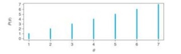
The random walk, would look like this:

• At time=1, you are in district 4.
• Flip a coin. The proposed move is to district 5.
• Accept the proposed move because the voter population in district 5 is greater than that in district 4.
• New day. Flip a coin. The proposed move is to district 6. Greater population, so you move.
• New day. Flip a coin. The proposed move is to district 7. Greater population, so you move.
• At time=4, you are in district 7. Flip a coin. If the proposal is to move to district 6, you base your decision to move on the probability criterion of 6/7. Draw a random sample between 0 and 1, if the value is between 0 and 6/7, you move. Otherwise you remain in district 7.
• Repeat many, many times.

Note in the figure above how the density of the moves begins to mirror (upside down) the distribution of voters. This next figure represents the amount of time you spend in any one district.

And the following figure illustrates the evolution of this distribution over time.

[]http://www.columbia.edu/~cjd11/charles_dimaggio/DIRE/resources/Bayes/Bayes2/(mcmc4.jpg)

You can see it gradually approaches the target distribution, even though the only information you have is from one step in either direction. Notice, also, the initial “bulge” of probability around the starting value of district 4. This is feature of MCMC, and why you will need to carefully consider initial or starting values for your simulations, and allow adequate “burn in” time.

The basis of the Metropolis algorithm, then, consists of: (1) proposing a move, and (2) accepting or rejecting that move. Proposing a move involves a proposal distribution. Accepting or rejecting the move involves an acceptance decision.

The proposal distribution is the range of possible moves. In the simple example with which we’ve been working, the proposal distribution consists of two possible moves: to the east or to the west, each with a probability of 50% based on the flip of a coin.

The acceptance decision for the proposal distribution is based on a probability. It is really quite clever:

\[ Pr[move] = P_{min} (\frac{P_{\theta_{proposal}}}{P_{\theta_{current}}}, 1) \]

So, if the population of the proposed district is greater than the current population, the minimum is 1, and you move with 100% certainty. If, on the other hand, the proposed population is less than the current population, you move with a probability equal to that proportion. The process works because the relative transition distributions match the relative values of the target distribution. You can summarize the process, from coin flipping to acceptance probability as

\[ 0.5*P_{min}(\frac{P_{\theta_{proposal}}}{P_{\theta_{current}}}, 1) \].

Because we are only interested in the ratio of the proposed to the current values, the final (target or posterior) distribution is not normalized. It does not have to integrate or sum up to 1, The consequence of this is that we are not restricted to closed solutions. We can use this approach to get at any complex posterior distributions or the kind \(Pr[data|\theta]*Pr[\theta]\)

From discrete Metropolis algorithm to continuous

The Metropolis algorithm can be generalized from the discrete (e.g. “right vs. left move”) case to a continuous multi-dimensional parameter space version while remaining essentially the same. As mentioned earlier, the main criterion is to be able to calculate the \(Pr[\theta]\) for any candidate value of \(\theta\). Since it doesn’t have to be normalized, i.e., all we need is the ratio of the proposed to the current , we can use the product of the likelihood and the prior to calculate the of the posterior.

A normally distributed proposal distribution makes it easier to generate proposal values, and the proposed move will typically be near the current position. The decision to move is based on the same probability as that in the simple discrete version:

\[ Pr[move] = P_{min}(\frac{P_{\theta-propose}}{P_{\theta-current}}, 1) \]

Some care needs to be taken in specifying a proposal distribution. If the proposal distribution is too narrow, it will take a long time to traverse the entire target distribution, especially if the initial or starting value is off somewhere in the hinterlands of a large multi-dimensional parameter space. That’s one reason that the operationalization of a Metropolis algorithm should involve more than one starting value. Of course, it’s also a potential problem if the proposal distribution is too wide. Then, \(\frac{P_{\theta-propose}}{P_{\theta-current}}\) will rarely be large enough to move from the current spot, and your sample will be “stuck” in a localized area of the target distribution.

Metropolis algorithm with two parameters

Let’s review and extend the Metropolis algorithm to the two-parameter setting. The mechanics of applying the Metropolis algorithm to a two-parameter bivariate normal model proceed similarly to the simple one-parameter setting. As a quick recap, our random walk starts at some arbitrary starting point, hopefully not too far away from the meatiest part of the posterior distribution. We propose a move from our current position using a proposal distribution from which (we assume) it is easy to generate values. We accept the move with certainty if the target or posterior distribution is more dense (of greater value) at the proposed position than at the current position. If the target or posterior distribution is less dense at the proposed vs. the current position, we accept the move with probability set to the ratio of the proposed to the current value.

The algorithm, then, needs only a few simple tools:

• a value sampled randomly from the proposal distribution
• another value sampled randomly from a \(\sim Unif(0,1)\) distribution to accept or reject probabilistic moves
• the ability to calculate the likelihood and prior for any given parameter values
  • conveniently, since we are only interested in their ratio, these values don’t have to be normalized

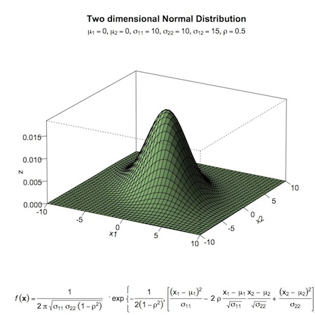
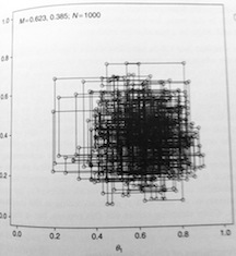
For a two-parameter problem, we can use the product of beta distributions as a prior. As an example (again, from John Kruschke’s text) of a two-parameter setting, we will work with a a bivariate normal proposal distribution. Below, you’ll find the proposal distribution and the R-code used to create it. Then the scatter plot of samples (excluding a burn-in period), where \(N_{pro}\) is the number of accepted proposals. Note that for more complex parameter spaces, it may be difficult or impossible to visualize your proposal distribution, but the underlying concepts remain the same.

1
2
3
4
5
6
7
8
9
10
11
12
13
14
15
16
17
18
19
20
21
22
23
24
25
26
27
28
29
30
31
32
33
34
35
36
37
38
39
40
41

 # R code to create bivariate figure
mu1<-0 # set mean x1
mu2<-0 # set mean x2
s11<-10 # set variance x1
s22<-10 # set variance x2
s12<-15 # set covariance x1 and x2
rho<-0.5 # set correlation coefficient  x1 and x2
x1<-seq(-10,10,length=41) # generate vector  x1
x2<-x1 # copy x1 to x2


f<-function(x1,x2) # multivariate function
{
term1<-1/(2*pi*sqrt(s11*s22*(1-rho^2)))
term2<--1/(2*(1-rho^2))
term3<-(x1-mu1)^2/s11
term4<-(x2-mu2)^2/s22
term5<--2*rho*((x1-mu1)*(x2-mu2))/(sqrt(s11)*sqrt(s22))
term1*exp(term2*(term3+term4-term5))
} 

z<-outer(x1,x2,f) # calculate density values


persp(x1, x2, z, # 3-D plot
main="Two dimensional Normal Distribution",
sub=expression(italic(f)~(bold(x))==frac(1,2~pi~sqrt(sigma[11]~
sigma[22]~(1-rho^2)))~phantom(0)^bold(.)~exp~bgroup("{",
list(-frac(1,2(1-rho^2)),
bgroup("[", frac((x[1]~-~mu[1])^2, sigma[11])~-~2~rho~frac(x[1]~-~mu[1],
sqrt(sigma[11]))~ frac(x[2]~-~mu[2],sqrt(sigma[22]))~+~
frac((x[2]~-~mu[2])^2, sigma[22]),"]")),"}")),
col="lightgreen",
theta=30, phi=20,
r=50,
d=0.1,
expand=0.5,
ltheta=90, lphi=180,
shade=0.75,
ticktype="detailed",
nticks=5) 

bivariate normal proposal distribution

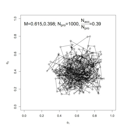
Metropolis scatter plot

Gibbs Sampling

As we have noted, for the Metropolis sampler to work well, the proposal distribution needs to be “tuned” to the poster distribution. If the proposal distribution is too narrow, too many proposed moves or samples will be rejected. If it is too wide, it can get bogged down in a local region and not move efficiently across the parameter space. Gibb’s sampling (Geman and Geman, 1984) is an alternative algorithm that does not require a separate proposal distribution, so is not dependent on tuning a proposal distribution to the posterior distribution.

The main difference between Gibbs sampling and Metropolis sampling is how the proposal value is chosen. Instead of choosing a proposed value from a proposal distribution that represents the entire multi-parameter density, the Gibbs sample chooses a random value for a single parameter holding all the other parameters constant. The randomly proposed single parameter is combined with the unchanged values of all the other parameters to calculate the proposed new position in the random walk. The Gibb’s sampler then repeats this process sequentially through all the parameters, calculating a proposal value, and accepting or rejecting it in turn. You can think of it as a special case of the more general Metropolis algorithm, where the proposal distribution is determined, at each step, by the conditioning variables. Note that the process is set up so that the proposal distribution will exactly mirror the posterior probability for a parameter. So, the proposed move is always accepted. This is why the Gibb’s sampler is more efficient than the Metropolis sampler. You may see references to the Metropolis-Hastings algorithm. This is a generalization of the Metropolis algorithm required to prove that the Gibbs sampler “works”.

To sum up Gibbs sampling:

• Select a parameter
• Choose a random value for that parameter from a conditional distribution based on all the other parameters
• The new point is determined by the values of the other parameters and the proposed value of the parameter conditional on them

Gibbs sampling is useful when the complete posterior distribution cannot be determined and so cannot be sampled. This may be the case in complex models. The following figure illustrates the concept for the two-parameter bivariate normal model.

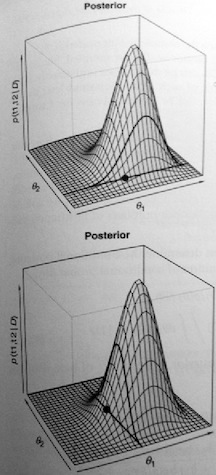
The top figure shows a randomly generated value of \(\theta_1|\theta_2\). The dark line is a slice through the posterior at the conditional value of \(\theta_2\). The dot is the value of \(\theta_1\) from that conditional distribution. The bottom figure shows the same process for \(\theta_2|\theta_1\). As opposed to the Metropolis algorithm, the Gibbs sampler results in the following scatterplot.

Programs like WinBUGS, OpenBUGS and JAGS, even though they are named for Gibbs sampling, often use Metropolis algorithms, or even conjugate results if available, depending on the model specification. You can override the default behaviors, but will rarely have reason to.

Implementing a Gibbs Sampler

Gibbs sampling arose to deal with messy joint posterior distributions where it is very difficult to sample from all the parameters in the joint space simultaneously. Rather than sample directly form a joint posterior distribution like \(Pr[(\mu_0, \sigma_0,\mu_1, \sigma_1, \alpha) |y]\), the Gibbs algorithm cycles through the conditional distributions for each parameter, e.g. e.g. \(Pr(\alpha | (\mu_0, \sigma_0,\mu_1, \sigma_1, y))\). So, given values for \(\mu_0, \sigma_0,\mu_1, \sigma_1, y\), we estimate \(\alpha\). Then, given values for \(\alpha ,\sigma_0,\mu_1, \sigma_1, y\), estimate \(\mu_0\). Then similarly cycle through the rest of the parameters, using the estimated value for a parameter for each subsequent step in the cycle, so that we are always using the most updated value. This process is repeated again and again (like an expectation-maximization algorithm) until we arrive or “converge” at a reasonable estimate of the full joint posterior distribution. ¹⁰

You can, if you like, think of Gibbs sampling in terms of an EM algorithm, which are used for mixture models to return optimal values for point estimates. For the “expectation” step, rather than “divide” an observation up into parts, with some of the observation in one of the underlying distributions and some in the other underlying distribution, the Gibbs sampler “flips” a coin based on the probability of an observation being in one of the underlying distributions or the other, and “moves” the observation entirely into that distribution. Then, for the “maximization” step, Gibbs uses that choice of the distribution for the estimate of the next parameter, e.g. \(p(\alpha|\sigma^2, \mu, I, y)\), then plugs that value into the formula to sample the next parameter conditional on the given parameters. In contrast to the EM algorithm, with Gibbs sampling we can explore the entire joint posterior probability space.

Gibbs sampling is very powerful, but the issue of convergence is critically important, and it is the responsibility of the analyst to diagnose convergence. One popular approach is to run multiple chains to ensure that sampler arrives at the same place regardless of where it starts. Another issue is autocorrelation. Simple sampling implementations in R (e.g. sample()) are independent. Markov Chain produces correlated samples because by definition the probability of subsequent events depends on the current state. We will need to evaluate how correlated the samples are, and perhaps “thin” them by including only every \(k^th\) observation in our sample.

The following R code presents Gibbs sampling for a target bivariate normal distribution. ¹¹ It runs through the process of setting up the sampler, running two chains from two different dispersed starting values, evaluating and addressing convergence (“burn-in”) and autocorrelation. We see the final results are very close to the target distribution, and that we can fully describe the distributions in terms of point estimate and spread.

1
2
3
4
5
6
7
8
9
10
11
12
13
14
15
16
17
18
19
20
21
22
23
24
25
26
27
28
29
30
31
32
33
34
35
36
37
38
39
40
41
42
43
44
45
46
47
48
49
50
51
52
53
54
55
56
57
58
59
60
61
62
63
64
65
66
67
68
69
70
71
72
73
74
75
76
77
78
79
80
81
82
83

numiters <- 10000

 # set means and covariances for bivariate normal
mu1 <- 0
mu2 <- 0
sigsq1 <- 1
sigsq2 <- 1
rho <- 0.9

 # set sampler to run from starting values theta1=10 and theta2=10
theta1 <- rep(NA,numiters)
theta2 <- rep(NA,numiters)
theta1[1] <- 10 # starting points for theta1 and theta2 in first chain
theta2[1] <- 10
for (i in 2:numiters){
  theta1[i] <- rnorm(1,rho*theta2[i-1],sqrt(1-rho^2)) # sample from conditional distribution
  theta2[i] <- rnorm(1,rho*theta1[i],sqrt(1-rho^2))
  print(i)
}


 ## set second different starting values theta1=-10 and theta2=-10
theta1.alt <- rep(NA,numiters)
theta2.alt <- rep(NA,numiters)
theta1.alt[1] <- -10 # starting point2 for theta1 and theta2 second chain
theta2.alt[1] <- -10
for (i in 2:numiters){
  theta1.alt[i] <- rnorm(1,rho*theta2.alt[i-1],sqrt(1-rho^2))
  theta2.alt[i] <- rnorm(1,rho*theta1.alt[i],sqrt(1-rho^2))
  print(i)
}

mintheta1 <- min(theta1,theta1.alt)
mintheta2 <- min(theta2,theta2.alt)
maxtheta1 <- max(theta1,theta1.alt)
maxtheta2 <- max(theta2,theta2.alt)

 ## plot first 100 iterations
par(mfrow=c(2,1))
plot(1:100,theta1[1:100],col=1,ylim=c(mintheta1,maxtheta1),type="l")
lines(1:100,theta1.alt[1:100],col=2)
plot(1:100,theta2[1:100],col=1,ylim=c(mintheta2,maxtheta2),type="l")
lines(1:100,theta2.alt[1:100],col=2)

 ## plot all 10000 iterations
par(mfrow=c(2,1))
plot(1:numiters,theta1,col=1,ylim=c(mintheta1,maxtheta1),type="l")
lines(1:numiters,theta1.alt,col=2)
plot(1:numiters,theta2,col=1,ylim=c(mintheta2,maxtheta2),type="l")
lines(1:numiters,theta2.alt,col=2)

 ## throw out first 100 as "burn-in", combine chains

theta1.new <- c(theta1[101:numiters],theta1.alt[101:numiters])
theta2.new <- c(theta2[101:numiters],theta2.alt[101:numiters])

numsamples <- length(theta1.new)

 # plot auto-correlation of each parameter

par(mfrow=c(2,1))
acf(theta1.new)  # acf() is R autocorrelation function
acf(theta2.new) 

 ## looks like correlation dies off after about 15th sample 
## (see on plot, upright correlation plot falls into the 
## little dashed blue line tick marks at about that number)
 ## keep independent samples by only taking every 15th sample:

temp <- 15*c(1:(numsamples/15))
theta1.final <- theta1.new[temp]
theta2.final <- theta2.new[temp]

 ## go from 20,000 samples (two chains of 10,000 each) 
to about 1,000 samples, but more confident they are independent and converged

par(mfrow=c(2,1))
acf(theta1.final)
acf(theta2.final) 

mean(theta1.final)
mean(theta2.final)
sd(theta1.final)
sd(theta2.final)
cor(theta1.final,theta2.final)

Gibbs vs. Metropolis

Gibbs sampling is (relatively) conceptually easy to implement because we are able to break up the non-standard joint posterior distributions into standard conditional probability distributions. This may not always be possible. For example, recall plane crash model with time trend for which we used grid sampling. The conditional distributions \(p(\alpha|\beta, y)\) and \(p(\beta|\alpha, y)\) are themselves non-standard, so we can’t sample directly from them using Gibbs sampling. We can, though, use the Metropolis algorithm.

In the Metropolis algorithm, instead of using a grid of all possible values, we again take a Markov chain approach and move from a current value to a subsequent value based solely on the current value. As with Gibbs, we start with a current value, but then we “propose” a new next value. If the newly proposed value has a higher posterior probability than the current value, we will be more likely to accept it move to it. If the newly proposed value has a lower posterior probability than the current value, we will be less likely to accept and move to it.

In practice, we start with a “proposal distribution”, e.g. \(\alpha^{proposal} \sim (Nl(\alpha^{current}, 1))\). We then make a decision to accept or reject a newly proposed value from that distribution based on $ r = \(. If \)r>1$ we will accept and move to new value with certainty. If \(r<1\), we “flip a coin” with the probability of accepting or moving to the new value move equal to \(r\). If that probability \(r\) is very small probability, we will not be very likely to accept and move to the new value, if relatively high, we are more likely to accept and make the move. So, rather than using a grid of possible values to evaluate the posterior space, we are “jumping around” the posterior probability space in a stochastic fashion. We never actually “see” or propose the whole space, but in the end, we will have a good description of it because we will explore it stochastically based on the probability of individually proposed values being in the space.

The Metropolis algorithm is more flexible than Gibbs, but comes with it’s own issues. There may be more problems with convergence and autocorrelation. It will generally run slower (sometimes much slower) than Gibbs, because of all those rejected values (Gibbs sampling doesn’t reject values, just calculates their probability). Much of the efficiency and speed will depend on our proposal distribution. The proposal distribution is centered on your current position, which is generally a good thing. But if we begin with a poor starting point, there will be many rejections early on, and it may take you a long time to get to more “meaty” areas of the distribution where we are more likely to accept values. (Early on, you will see runs of horizontal lines of “rejections” in convergence plots.) The variance of the convergence distribution also plays an important role in how quickly the sampler will explore the posterior probability space. “Tuning” or adjusting the variance of the proposal distribution may be necessary to get your sampler to converge more quickly.

Assessing MCMC Runs

There are issues to consider with MCMC methods that don’t arise in classical statistical inference. In addition to more familiar aspects of statistical analysis, the process of conducting an MCMC analysis involves assessing graphs and diagnostics for convergence, mixing, acceptance rates or efficiency, and correlation. Specifically, you’ll explore convergence or whether your sample of \(\theta\) ’s approaches the posterior distribution of \(Pr(\theta | y)\)), “mixing”, i.e. whether the sampler algorithm explored the entire posterior distribution, efficiency or how well \(Pr(\theta | y)\) is estimated by the sample of \(\theta\) ’s you’ve generated or whether you need a larger sample size, and autocorrelation of the values in your sample.

Convergence

Convergence in MCM refers to the final, stable set of samples from the target or “stationary” posterior distribution. A series of samples, “converges” to a distribution, not a particular value. The series of samples or iterations that precedes convergence is sometimes referred to as “burn in”. Once convergence is achieved, samples should look like random scatter around a stable mean.

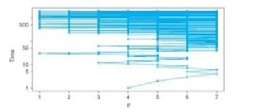
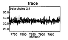
You have an obligation when conducting MCMC to assess convergence. But, there is no fool-proof means of assuring convergence. Sometimes, all that is needed is a graphical assessment of trace plots by iteration number for multiple chains starting from dispersed initial values. For example, look at two chains on a trace plot for the quick, jerky or spiky overlapping chains indicative that they are both sampled from the same space.

Convergence

Some statistical tests (available in CODA and BOA R software packages) may help diagnose convergence. One popular test is is the Gelman-Rubin statistic, which compares multiple chains, each with widely differing starting points, by quantifying whether sequences are farther apart than expected based on their internal variability.

Problems with convergence

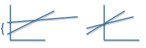
You may find that it takes an inordinately long period of time for your samples to converge to a stable distribution. Or that the samples never converge. This may be due to correlation between variables in your model. On the figure on the left (below) you see small changes in one variable are associated with large changes in the other variable. The MCMC algorithm will have to sample a largely dispersed probability space, and it may not do this quickly or perhaps at all. One possible fix is to “center” the variables, e.g. by subtracting the mean, or standardizing. Centering doesn’t change the relationship between variables, it just moves the intercept, resulting in a situation like that on the right side of the figure. Now, the MCMC algorithm will run and converge more quickly because it has only to sample from a relatively tight probability space.

NonConverge

Efficiency

After your sampling algorithm has converged to an acceptably stable, stationary posterior distribution, you will need further iterations to obtain samples for posterior inference. The more iterations you sample, the more accurate the posterior estimates. But, since the sample is not independent, you can’t use traditional standard error estimates. Instead, you can assess the efficiency or accuracy of your estimates with a Monte Carlo standard error, which is the standard error associated with the posterior sample mean as a theoretical expectation for a given parameter. As noted above, the MC error is calculated as \(\frac{\sigma^2_{sample}}{\sqrt{n_{iterations}}}\), and depends on:

• the true variance of the posterior distribution,
• the posterior sample size (i.e. the number of MCMC iterations)
• autocorrelation in the MCMC sample.

As a rule of thumb, you’d like to see an MC error less than 1% to 5% of your posterior standard deviation.

Autocorrelation

Since a sample value at time t is based on the previous value at time t-1 , the samples will invariably be correlated. It is, actually less of a concern than you might expect, because your inferences and summary measures are based on the entire sample taken together, not on the series. Still you’d like the correlation to be small as possible, with a relatively steep drop off as the lag number increases indicating convergence to independent samples. This also increases efficiency because you can explore the entire probability space as efficiently as possible with as small a sample as possible. You can assess correlation in your sample chain with autocorrelation plots (autocorrelation by lag time), with the goal of autocorrelation decreasing to zero in as few steps as possible.

Running MCMC in BUGS

The BUGS Program ##3

BUGS stands for Bayesian inference using Gibbs sampling. It’s a language for specifying complex Bayesian models. WinBUGS and it’s open-source cousin OpenBUGS are perhaps the first and most well-known implementations, but since I started using a Mac I’ve migrated over to JAGS (Just Another Gibbs Sampler) because of it’s cross-platform ease of use. To follow along with the material below you will need to download the software at the links above, and install R2WinBUGS, R2OpenBUGS and/or R2jags packages from CRAN.

WinBUGS was originally distinguished form other implementations of Gibbs sampling by the use of graphical object-oriented internal representations of models called “Doodles”. The “Doodle Editor” allows you to create models graphically and can be very nice to work with, though I don’t know many folks who use it. Most folks find themselves using the the point-and click-approach built into Win/OpenBUGS. This consists of:

1. Specifying a model (We’ll talk about this in a moment)
2. Double clicking the word “Model” to select it
3. Clicking “Check Model” in the menu (under “Model > Specification…”)
4. Look for the message in the lower left hand side of you screen that your “model is syntactically correct”
5. Clicking “Compile” (again under under “Model > Specification…”, and again checking the message that your “model compiled”)
6. Clicking “load inits” (or “gen inits” if you are allowing WinBUGS to generate initial values for you) under the same menu and looking for the to load or generate initial or starting values for your MCMC algorithm, and again monitoring the response, this time that your “model initialized”
7. Loading your data (under the same menu)
8. Clicking “Samples” under the “Inference” menu to specify the beginning (“beg”) and ending (“end”) for your the number of iterations or samples on which you want to base your results (here is where you can specify your “burn-in” period)
9. Typing the names of the “nodes” (parameters) you want results for in the “Sample Monitor” window, clicking “Set” after entering each node
10. Clicking on “Update” in the menu to specify the total number of iterations and begin the MCMC process
11. Clicking (again) on “Samples” under the “Inference” menu
12. Typing “*” in the “Sample Monitor”and clicking “Stats” to see results
13. Typing “*” in the “Sample Monitor”and clicking “Trace” to see sampled values
14. Clicking on various diagnostics and tools like “bgr statistic” for the Gelman-Rubin statistic
15. Clicking on various plots and graphs to assess convergence and autocorrelation

If this seems like a lot of pointing and clicking, well, it is. Most folks quickly tire of it. The good news is that you can run the entire process under R with some fairly simple interfaces to your BUGS program of choice. Perhaps the most popular of this syntax-driven approach is to interface BUGS with R using the R2WinBUGS package. Although, as I say above, my preference is the R2jags package.

Specifying a Model

Before going over how to specify a model in R, we need to discuss how to specify a model. We’ll begin with a simple example using the point-and-click approach described above. It will allow you to see native BUGS software, and likely convince you that you no longer wish to work with native BUGS software. We’ll recreate the coin toss example from the top of the page that we coded in R. We are interested in the probability of 8 or more heads in 10 tosses of a fair coin. Our outcome, y, is ~Bernoulli(0.5, 10) The model statement for this problem in BUGS is:

Model{
Y ~ dbin(0.5, 10)
P8 <- step(Y-7.5)
}

BUGS doesn’t have the capability for “if-then” statements, so we use a step function instead. If the argument is true, it returns a value of 1, otherwise it returns a value of 0. Here we are saying that if Y-7.5 is greater than or equal to zero (i.e. Y is 8 or more) P8 takes on the value 1, otherwise P8 takes on the value 0. We assign the results of the step function to an indicator variable called P8 so we can monitor and get results on it. Cut and paste this model into an new model frame in Win or Open BUGS and go through the the point-and-click approach outlined above. Let WinBUGS generate initial values. And, since this is pure Monte Carlo, you don’t need to load any data. Run 5000 iterations and monitor the results of the P8 variable. When you (finally) click on “stats” in the “sample monitor tool” you should get something like:

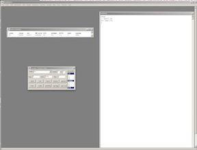
WinBUGS Screen Shot

The BUGS Language:

In some statistical software programs, you tell the package where the data is and it applies pre-packaged statistical models. Like R, WinBUGS is much more flexible. You can specify just about any model you like, and then apply your own model to the data. The model language itself is similar to R. So, <- represents logical dependence e.g. m <- a+ b*x. Unlike R, though, the tilde symbol (~) represents a stochastic or probability dependence, e.g x ~ dunif(a,b). One very important point about specifying probability distributions in BUGS: you define distributions in terms of precision, not variance, so ~ dnorm(0.0,1.0E-6) means a very small precision, and a very wide (in this case almost uniform) variance.

Arrays and loops are also similar to R language:

for (i in 1:n){
r[i] ~ dbin(p[i], n[i])
p[i] ~ dunif(0,1)
}

BUGS comes with functions, some of which may be familiar, e.g.

mean(p[])

returns the the mean of a whole array,

mean(p[m:n]) 

returns the mean of elements m to n.

Some (but not all) of functions can appear on the left side of an expression, e.g.

logit (p[i]) <- a + b*x[i]
log(m[i]) <- c + d*y

Here are some useful BUGS functions:

p<-dnorm(0,1)I(0,) 

Truncates the variable, which means the variable will be restricted to the range 0 to infinity (i.e. only the positive side of a normal distribution). This can be useful when specifying a prior distribution that can not, say, have negative values.

p<- step(x-1) 

Returns a 1 if x is greater than or equal to 1 (or any number), and a 0 otherwise. Monitoring p and recording it’s mean will give the probability that x is greater than or equal to 1.

p<- equals(x, .7)

Does the same thing for x equal to 1.

tau <- 1/pow(s,2)

Sets \(\tau\) to \(\frac{1}{s^2}\)

complex functions as parameters

Since in a Bayesian model both variables and parameters are allowed to vary and are associated with errors, you can construct and calculate errors for even the most complex functions. You just calculate the the function as a node at each iteration and summarize the posterior samples as you would for any node. Practically, this involves adding in extra lines of code to monitor what you’re interested in. For example, suppose you are interested in the the dose of a drug that will provide 95% efficacy (“ED95”). In BUGS you can add a line of code like this:

ED95 <- (logit(0.95) – alpha) / beta

Where, alpha is the intercept or baseline response and beta is the change in response per unit dose.

Similarly, you could enter a missing or predicted value using your model, and monitor results for that. For example, say you model the effect of distance from a disaster (x1), local deaths from that disaster (x2) and median household income (x3) on psychological distress. Your BUGS statement for the model could be:

y[i] <- beta0 + beta1 * x1[i] + beta2*x2[i]  + beta3*x3[i] 

You can enter and model the results of the effect of 2, 4 and 6 mile distances with a few lines of code, substituting the mean values for the other two variables (x2 and x3), and monitoring and summarizing the new variables y2, y4, y6.

y2 <- beta0 + beta1 * 2 + beta2*1.26  + beta3*41064 
y4 <- beta0 + beta1 * 4 + beta2*1.26  + beta3*41064 
y6 <- beta0 + beta1 * 6 + beta2*1.26  + beta3*41064 

Airline fatality data example

Now, let’s look at an example of running a Bayesian MCMC analysis by interfacing R to a BUGS program. As I mentioned above, I prefer to use the JAGS program and interface with the R2jags package, but you can do the same thing (and should get the same answers) using WinBUGS with R2WinBUGS, or OpenBUGS with R2OpenBUGS.

This example comes from Lyle Gurrin and Bendix Cartensen We are going to analyze 26 years worth of airline fatality data using a simple Poisson model that will allow us to compare the exact form of the posterior to the simulated MCMC results.

Begin by reading in the airline fatality data. which you can find here.

1
2

airline<-read.csv("~/airline.csv",header=T, stringsAsFactors=F)
airline

Explore the airline data, then take advantage of conjugacy to get the exact results for the posterior distribution for the mean number of fatalities. The model for the data or likelihood is \(y_i|\mu \sim Poisson(\mu)\). An uninformative prior for this data is \(\mu \sim \Gamma(0,0)\). For computational purposes we will use \(\mu \sim \Gamma(0.01,0.01)\) which is nearly uniform on \((0, +\inf)\). The conjugate posterior is then \(\mu \sim \Gamma(0.01 + \Sigma y_i, 0.01 + n)\), where \(\Sigma y_i\) is the total number of fatalities, and \(n\) is the number of observations.

Our result is the mean of the distribution, which we plot.

1
2
3
4
5
6
7

nrow(airline)
sum(airline$fatal)
head(airline)

(mn <- mean( xx <- rgamma( 10000, 634.01, 26.01 ) ) )
curve(dgamma(x,634.01,26.01), from=20, to=30, lwd=2)
abline( v=mn, col="red", lwd=3 )

Now, let’s compare this same value using MCMC simulation and BUGS (JAGS flavor in this case). We begin by creating a list object to hold the data, and another list object to hold the initial values for the simulation (notice that we need three values because we will be running three chains). We then write a model statement to file using the cat() function.

1
2
3
4
5
6
7
8
9
10
11
12
13
14
15
16
17
18

a.dat<-list(fatal=c(airline$fatal,NA), I=27)

a.inits<-list(
    list(mu=20),
    list(mu=23),
    list(mu=26)
    )

cat(
"model
{
for(i in 1:I)
{
fatal[i]~dpois(mu)
}
mu~dgamma(0.1,0.1)
}",
file="m1.jag")

We run the simulation in JAGS via the R2jags package function jags(). Type ?jags to get more information on options and use. We are essentially specifying with syntax, using the R objects we created, everything we had to point to and click on in WinBUGS. Note that we are only monitoring the parameter “mu”. Type ?jags to get more information on options and use.

1
2
3
4
5
6
7
8
9
10
11
12
13
14
15
16
17
18
19
20
21

library(R2jags)

args(jags)

res<-jags(data=a.dat, 
    inits=a.inits, 
    parameters.to.save="mu", 
    model.file="m1.jag")

print(res)
plot(res)
traceplot(res)

res.mcmc<-as.mcmc(res)
summary(res.mcmc)
plot(res.mcmc)

autocorr.plot(res.mcmc)

res.list<-mcmc.list(res.mcmc[[1]],res.mcmc[[2]],res.mcmc[[2]])
gelman.diag(res.list)

The summary, print, plot and traceplot functions operate directly on the bugs object R2jags produces. You’ll see that print() returns the statistics for the nodes we are monitoring. The plot() method returns some minimalist graphics summarizing the results. The traceplot() method returns plots for the three chains for each variable, here devaiance and mu. Each chain is in a different color. Notice how the chains are spiky, dense and overlapping, indicating convergence and good mixing.

We can get more tools by using the “coda” package. To access the tools in in the coda package, we first have to convert the jags object to an mcmc object. With the mcmc object, we can get the Gelman-Rubin statistic and autocorrelation plots, both of which look acceptable.