
Bayesian Analysis for Epidemiologists III: Regression Modeling
Acknowledgements
Much of this material comes from a workshop run by Drs. David Spiegelhalter and Nicky Best in Cambridge, UK, in 2005. Other major contributions come (again) from Lyle Gurrin and Shane Jensen.
Jim Albert
David Spiegelhalter
Nicky Best
Andrew Gelman
Bendix Carstensen
Lyle Guerrin
Shane Jensen and Statistical Horizons
Sections
I. Introduction to Bayesian Regression Modeling
1. Normal Model with Non-Informative Prior (Ridge or Penalized Regression)
2. Normal Model with Informative Priors (Lasso Regression)
3. Mixture Models (Expectation-Maximization)
II. Bayesian Regression Modeling with BUGS or JAGS
1. Linear Regression
2. Logistic Regression
3. Other Models
4. Hierarchical Models
Introduction to Bayesian Regression Modeling
Some of the advantages of using a Bayesian approach to statistical modeling is you can:
- include prior knowledge and “learn” from existing evidence
- easily extend to non-linear regression models
- easily make inferences and predictions by including complex functions of prior model results
- handle missing data directly in the model specification
- directly report results in terms of probability 1
Normal Model with Non-Informative Prior (Ridge or Penalized Regression)
A first approach to Bayesian regression modeling builds off the normal model, \(y_i \sim Normal(\mu, \sigma^2)\), by specifying \(\mu\) as a function of covariates, \(y_i \sim Normal(x_i \beta_i, \sigma^2)\). We might, for example, be interested in body weight as a linear function of abdominal and wrist circumference. Classical regression becomes Bayesian when we put priors on our parameters \(\beta\) and on \(\sigma^2\). 2
Non-informative priors return results very close to classical statistics. The approach is similar to the normal model we have already seen, where \(p(\mu) \propto 1\) is flat on \(\mu\), and \(p(\sigma^2) \propto (\sigma^2)^{-1} \) is flat on the of \(p(\sigma^2)\). Only now, we apply the prior to all the coefficients: \(p(\beta_i) \propto 1\), which results in a more complicated joint posterior:
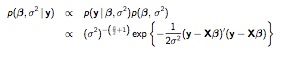
NlRegJointPost
We (again) use a two-step approach, first sampling the conditional posterior for \(\beta\) given \(\sigma^2\) (and the data), then sampling the marginal posterior of \(\sigma^2\) given the data. 3
As opposed to the classical framework where prediction is based on a single value of \(\hat{\beta}\),\(y* \sim Normal(\hat{\beta}, \sigma^2)\), in the Bayesian approach, we will include additional uncertainty of \(\beta_i\), \(p(\beta|\sigma^2,y)\) which is that Inverse Gamma distribution we saw in the normal model, the expectation or mean of which ends up being \(\Sigma(y_i - X_i \hat{\beta})^2/n-p\). So, again, the predictive interval in the Bayesian framework is potentially much wider than that from classical regression. This Bayesian regression with normally distributed priors for the coefficients centered at zero, is sometimes referred to as ridge or penalized regression.
In practical application, as before, we incorporate the additional uncertainty by using samples of \(\beta_i\) in the calculation of y*, the general scheme of which is:
- Sample \(\sigma^2\) from the Inverse Gamma distribution.
- Feed those values into a simulation to sample \(\beta\)
- Use the simulated sample values of \(\sigma^2\) and \(\beta\) to arrive at a distribution of values for y*
- Summarize y*
Again, as a practical matter, in this setting of a non-informative prior, we can take advantage of the fact that the point estimates for the Bayesian and ordinary least squares approaches are the same. We will simply run a classical linear model (e.g. in R using lm()), then use those results for for the simulations and probability calculations that allow the coefficients to vary and account for additional variability in the predictions. We see this approach in the following sample code 4 predicting tree volume based on tree girth and height.
1 2 3 4 5 6 7 8 9 10 11 12 13 14 15 16 17 18 19 20 21 22 23 24 25 26 27 28 29 30 31 32 33 34 35 36 37 38 39 40 41 42 43 44 45 46 47 48 49 50 51 52 53 54 55 56 57 58 59 60 61 62 63 64 65 66 67 68 69 70 71 72 73 74 75 | data(trees) attach(trees) trees ## Plotting Outcome (Volume) as a function of Covariates (Girth, Height) par(mfrow=c(1,2)) plot(Girth,Volume,pch=19) plot(Height,Volume,pch=19) ## MLE fit of Regression Model model <- lm(Volume~Girth+Height) summary(model) par(mfrow=c(1,1)) plot(model$fitted.values,model$residuals,pch=19) abline(h=0,col=2) ## Sampling from Posterior Distribution of coefficients beta and variance sigsq beta.hat <- model$coef n <- length(Volume) p <- length(beta.hat) s2 <- (n-p)*summary(model)$sigma^2 V.beta <- summary(model)$cov.unscaled numsamp <- 1000 beta.samp <- matrix(NA,nrow=numsamp,ncol=p) sigsq.samp <- rep(NA,numsamp) for (i in 1:numsamp){ temp <- rgamma(1,shape=(n-p)/2,rate=s2/2) cursigsq <- 1/temp curvarbeta <- cursigsq*V.beta curvarbeta.chol <- t(chol(curvarbeta)) z <- rnorm(p,0,1) curbeta <- beta.hat+curvarbeta.chol%*%z sigsq.samp[i] <- cursigsq beta.samp[i,] <- curbeta } ## Plotting Posterior Samples for coefficients beta and variance sigsq par(mfrow=c(2,2)) hist(beta.samp[,1],main="Intercept",col="gray") abline(v=beta.hat[1],col="red") hist(beta.samp[,2],main="Girth",col="gray") abline(v=beta.hat[2],col="red") hist(beta.samp[,3],main="Height",col="gray") abline(v=beta.hat[3],col="red") hist(sigsq.samp,main="Sigsq",col="gray") abline(v=summary(model)$sigma^2,col="red") ## Posterior Predictive Sampling for new tree with girth = 18 and height = 80 Xstar <- c(1,18,80) # new tree with girth = 18 and height = 80 Ystar.samp <- rep(NA,numsamp) for (i in 1:numsamp){ Ystar.hat <- sum(beta.samp[i,]*Xstar) Ystar.samp[i] <- rnorm(1,mean=Ystar.hat,sd=sqrt(sigsq.samp[i])) } ## Plotting Predictive Samples and Data on same scale par(mfrow=c(2,1)) xmin <- min(Volume,Ystar.samp) xmax <- max(Volume,Ystar.samp) hist(Volume,main="Tree Volume in Observed Data",xlim=c(0,90),breaks=10,col="gray") abline(v=mean(Volume),col=2) hist(Ystar.samp,main="Predicted Volume of Tree with |
Normal Model with Informative Priors (Lasso Regression)
We are not limited to non-informative priors for our normally distributed linear Bayesian regression models. A conjugate prior for \(\beta\)’s in a normal model is also normal, \(\beta_k \sim Normal(\beta_{k0}, \tau^2)\), where, again, \(\tau^2\) is a measure of our confidence in the center of our prior distribution, \(\beta_{k0}\), and (again) as \(\tau^2\) approaches infinity, the prior approaches the non-informative prior above. We can take advantage of informative priors on the \(\beta\)’s to help identify and select coefficients for inclusion in model. We may, for example, have a set of high-dimensional data, where there are many more coefficients than outcomes. This is often the case in analysis of medical imaging data like MRI’s where each image is characterized by many potentially important variables, but there are only a limited number of patients or outcomes. We may believe that only a small subset of the many potential variables are important, but we don’t know which ones. By setting all priors on all the \(\beta\) coefficients to zero, and making \(\tau^2\) small to reflect high confidence that most of the coefficients are unimportant, we can identify and select out only those coefficients strongly supported by the data.
A currently popular method sometimes referred to as Lasso Regression is essentially a Bayesian regression with (informative) Laplace priors placed on the \(\beta\) coefficients. A Laplace prior looks like two exponential distributions back to back. It constrains the area around, and places a stronger confidence on zero than does a normal prior centered on zero.
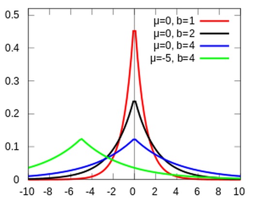
LaplacePrior
Mixture Models
Sometimes a single set of data arise from two different processes. Take, for example, home runs in major league baseball. The large majority of professional players won’t hit many home runs, perhaps 10 in a season. A subset of elite home run hitters will hit many more. You can think of it as data from two normal distributions, one with a mean lower than the other, mixed together. Some of the data, \(y_i\), from a normal distributions with mean \(\mu\)_0 and standard deviation \(\sigma_0\) with probability \(\alpha\). The data from the other normal distribution has a different mean \(\mu_1\) and \(\sigma_1\) with prob \(1-\alpha\). (The probability \(\alpha\) is sometimes referred to as the mixing proportion.) If you could identify which distribution the observations come from, you could split them up and analyze them separately. But you can’t. An observation could, for example, be coming from an elite hitter having a bad year, or a mediocre hitter having a good year. 5
We are confronted with 5 unknown parameters: \(\mu_0\), \(\sigma_0\), \(\mu_1\), \(\sigma_1\), and \(\alpha\). We could put a flat, non-informative prior on each of them, but the resulting posterior involves the products of sums and is complicated and non-standard.
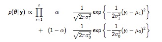
MixturePosterior
Taking the derivative for the MLE would be essentially impossible. Grid sampling with with 5 unknown parameters, we would require a 5-dimensional grid, which translates to \(100^5\) for just for 100 values. We will, instead, use an optimization algorithm called the (EM). The basic idea is to come up with additional data that would allow us to make the estimation problem easier. In this case, an indicator variable for which group the observations came from would do the trick. Of course, the problem in the first place is that we don’t have those indicators. But, the EM algorithm allows us to estimate these indicators for every observation, and then use those estimates. We proceed in two steps: expectation and maximization.
- The expectation step:
Start with some arbitrary values, e.g \(\mu_0 =5, \sigma_00.5,\mu_1=20, \sigma_1=0.5, \alpha=0.5\)
For each observation calculate the expectation using the starting values for the parameters
The expectation for an indicator variable is just the probability of the indicator variable being 1: \(E(I|\theta) = P(I=1|\theta)\)
For observations at the extremes of the curve, the probability could be clear enough to put the observations into one group of the other
For those observations where the probability is not so clear, split the observation up based on probability, with part of the observation in one group, and part of the observation in the other group
- The maximization step:
Once the total group of \(y_i\)’s is fractionated or segmented using the expectation step, calculating the MLE becomes much easier. The the posterior term becomes a much less complicated single product, not the sum of products.
Use the estimates for each of the parameters from the first pass (which were based on arbitrary choices) in a new expectation step for the indicators. Then, use those new indicators in another maximization MLE step for a second set of parameter estimates.
Use that second set of parameter estimates to get a third set of indicators, and feed those to the maximization step for a third set of parameters.
Lather, rinse, repeat. Basically a “hill climbing” algorithm that will run until convergence.
NB: Covariates could help inform and move the process along, e.g. player’s weight, \(\beta\).
In the following example from Shane Jensen’s course, first simulate a “true” underlying data set of a mixture of two normally distributed distributions, one with a mean of 0, the other with a mean of 4. Then pretend you don’t know that. Plotting the observed data indicates there may be two underlying processes going on.
The expectation function uses variables for the five unknown parameters to calculate the probability that an observation comes from one distribution or the other. The maximization function computes values for the five unknown parameters based on the results of the expectation function. Choose a reasonable value for each of the parameters to start the algorithm. Then set up a a while() loop with stopping rules to run through iterations of the estimation and maximization steps.
Plot the value for each parameter vs the number of iterations to see if and at what value the the algorithm settled into a stationary pattern. Extract point estimates for each of the four unknown parameters. Repeat the process using different starting values to check if we arrive at the same answers. (We should, and do.) Finally, compare our computational estimates to the true underlying values. (Something we will never be able to do in real life.)
1 2 3 4 5 6 7 8 9 10 11 12 13 14 15 16 17 18 19 20 21 22 23 24 25 26 27 28 29 30 31 32 33 34 35 36 37 38 39 40 41 42 43 44 45 46 47 48 49 50 51 52 53 54 55 56 57 58 59 60 61 62 63 64 65 66 67 68 69 70 71 72 73 74 75 76 77 78 79 80 81 82 83 84 85 86 87 88 89 90 91 92 93 94 95 96 97 98 99 | ## simulated data mixture of two normals with mu0=0,mu1=4,sigsq0=1,sigsq1=1,alpha=0.75 n <- 500 y <- rep(NA,n) ind.true <- rep(NA,n) for (i in 1:n){ ind.true[i] <- rbinom(1,1,prob=0.75) if (ind.true[i]==1){ y[i] <- rnorm(1,mean=4,sd=sqrt(1)) } if (ind.true[i]==0){ y[i] <- rnorm(1,mean=0,sd=sqrt(1)) } } ## plot observed data par(mfrow=c(1,1)) hist(y,col="gray") ## Expectation function: Estep <- function(alpha,mu0,mu1,sigsq0,sigsq1){ ind <- rep(NA,n) for (i in 1:n){ prob0 <- (1-alpha)*dnorm(y[i],mean=mu0,sd=sqrt(sigsq0)) prob1 <- alpha*dnorm(y[i],mean=mu1,sd=sqrt(sigsq1)) ind[i] <- prob1/(prob0+prob1) } ind } ## Maximization function Mstep <- function(ind){ alpha <- sum(ind)/n mu1 <- sum(ind*y)/sum(ind) mu0 <- sum((1-ind)*y)/sum(1-ind) sigsq1 <- sum(ind*((y-mu1)^2))/sum(ind) sigsq0 <- sum((1-ind)*((y-mu0)^2))/sum(1-ind) c(alpha,mu0,mu1,sigsq0,sigsq1) } ## starting values for EM algorithm: curalpha <- 0.5 curmu0 <- -1 curmu1 <- 1 cursigsq0 <- 1 cursigsq1 <- 1 itermat <- c(curalpha,curmu0,curmu1,cursigsq0,cursigsq1) ## run EM algorithm diff <- 1 numiters <- 1 while (diff > 0.0001){ # criterion to stop algorithm numiters <- numiters+1 curind <- Estep(curalpha,curmu0,curmu1,cursigsq0,cursigsq1) curparam <- Mstep(curind) curalpha <- curparam[1] curmu0 <- curparam[2] curmu1 <- curparam[3] cursigsq0 <- curparam[4] cursigsq1 <- curparam[5] itermat <- rbind(itermat,curparam) diff <- max(abs(itermat[numiters,]-itermat[numiters-1,])) print (numiters) } par(mfrow=c(2,3)) plot(1:numiters,itermat[,1],type="l",xlab="iters",ylab="alpha",main="alpha") plot(1:numiters,itermat[,2],type="l",xlab="iters",ylab="mu0",main="mu0") plot(1:numiters,itermat[,3],type="l",xlab="iters",ylab="mu1",main="mu1") plot(1:numiters,itermat[,4],type="l",xlab="iters",ylab="sigsq0",main="sigsq0") plot(1:numiters,itermat[,5],type="l",xlab="iters",ylab="sigsq1",main="sigsq1") theta.hat <- itermat[numiters,] theta.hat ## EM algorithm with different starting values: curalpha <- 0.5 curmu0 <- -10 curmu1 <- 10 cursigsq0 <- 2 cursigsq1 <- 2 itermat <- c(curalpha,curmu0,curmu1,cursigsq0,cursigsq1) ## calculate optimal density fit xgrid <- ppoints(1000)*10-2 yfit <- theta.hat[1]*dnorm |
In most realistic situations, the different mixtures will probably not be as obvious as they are in this example. They may, instead, look more like a normal distribution that appears to have too much information in one of the tails, or perhaps even like a truncated Poisson distribution.
Bayesian Regression Modeling with BUGS or JAGS
In this section we introduce how to model complex data using BUGS or JAGS. The “trick” (if there is one) is to discern the two main parts of a Bayesian model: the likelihood, and the priors. The rest tends to be tuning the machinery.
As a general approach, to conduct linear regression in the BUGS or JAGS you specify:
- the likelihood for the data
- the form of the relationship between response and explanatory variables
- prior distributions for regression coefficients and any unknown (nuisance) parameters
Linear Regression
Classical linear regression can be represented as:
\[ y_i = \beta_0 + \Sigma \beta_x * x_i + \epsilon \\ \epsilon \sim N(\mu, \sigma^2) \]
The Bayesian version can be represented as:
\[ y_i \sim N(\mu, \sigma^2) \\ \mu = \beta_0 + \Sigma \beta_x * x_i \\ \beta_x \sim priors \]
Note (importantly) that choosing so-called non-informative priors for \(\beta\) , like \(\beta_x \sim N(0, 10000)\) , and for the precision term, like \(\frac{1}{\sigma^2} \sim \Gamma(0.001, 0.001)\) will return classical or MLE results.
Example: New York City Crime Data
As an example of a Bayesian linear regression model, we look at New York City crime data from 1966 to 1967. The outcome variable (THEFT) is the increase or decrease in the seasonally adjusted rate of grand larcenies in 23 Manhattan police precincts from a 27-week pre-intervention period compared to a 58-week intervention period. The predictor variables are the percent increase or decrease in the number of police officers in a precinct (MAN), and whether the precinct was located uptown, midtown or downtown.
We specify the model as:
\[ THEFT_i \sim N(\mu, \sigma^) \\ \mu = \beta_0 + \beta_1 * MAN + district \\ \frac{1}{\sigma^2} \sim \Gamma(0.001, 0.001) \\ \beta_0 \sim N(0, 100000) \\ \beta_1 \sim N(0, 100000) \]
We will need a prior for the effect of geographic area (district), but will discuss that in a moment. First, we consider how best to code an indicator variable in BUGS. There are two possible approaches. We can create a “design matrix” of dummy variables. In this approach we create two variables named DIST1 and DIST2, for which downtown precincts are coded \(0,0\), midtown precincts are coded \(1,0\), and uptown precincts are coded \(0,1\). The BUGS code for this model would then be:
model{
for (i in 1:N) {
  THEFT[i] ~dnorm(mu[i] , tau)
  mu[i] <- beta0 + beta1*MAN[i] + beta2*DIST2[i] + beta3*DIST3[i]
}
beta0 ~dnorm(0, 0.00001)
beta1  ~dnorm(0, 0.00001)
beta2 ~dnorm(0, 0.00001)
beta3 ~dnorm(0, 0.00001)
tau ~ dgamma (0.001, 0.001)
sigma2 <- 1/tau}
Initial values for single chain for this model could be:
list(beta0 = 1, beta1 = -2, beta2 = -2, beta3 = 4, tau = 2)
Alternatively, we can code geographic area as a single vector, with \(1\) for downtown, \(2\) for midtown, and \(3\) for uptown. This, though, requires a little indexing slight of hand in the BUGS model specification. We will have to use the “double indexing” feature of BUGS:
model{
for (i in 1:23) {
  THEFT[i] ~dnorm(mu[i] , tau)
  mu[i] <- beta0 + beta1*MAN[i] + beta2*[DIST[i]] # or nested index
}
beta0 ~dnorm(0, 0.00001)
beta1  ~dnorm(0, 0.00001)
beta2[1]<-0       # reference category to make model identifiable
beta2[2] ~dnorm(0, 0.00001)
beta2[3] ~dnorm(0, 0.00001)
tau ~ dgamma (0.001, 0.001)
sigma2 <- 1/tau}
Initial values for a single chain for this model could be
list(beta0 = 1, beta1 = -2, beta2 = c(NA, -2, 4), tau = 2)
Let’s run the model with JAGS. We’ll use the design matrix approach to specify the indicator variable. Here, we read in the data (which I extracted from a pdf of the original Rand). JAGS likes named lists for data structures (though, I’ve found data frames to work just as well), so I create one with just the variables I plan to include in the model (JAGS will throw a warning if there are unused variables, but will otherwise run the model). I use the cat() function to hold the model syntax in a file called “m1.jag”. For simplicity, this syntax saves the file in the current working directory, but I could have saved it anywhere. Then I create a list object to hold the initial values (I’ve found JAGS like a list of lists), and a vector to hold the list of parameters I want to monitor. Finally, I load the R2Jjags package, and specify and run the model.
1 2 3 4 5 6 7 8 9 10 11 12 13 14 15 16 17 18 19 20 21 22 23 24 25 26 27 28 29 30 31 32 33 34 35 36 37 38 39 40 41 42 43 44 45 46 47 48 49 50 51 52 53 54 | PCT<- c(1, 4, 5, 6, 7, 9, 10, 13, 14, 16, 17, 18, 19, 20, 22, 23, 24, 25, 26, 28, 30, 32, 34) MAN<- c(-15.79, 0.98, 3.71, -5.37, -10.23, -8.32, -7.80, 6.77, -8.81, -9.56, -2.06, -0.76, -6.30, 39.40, -10.79, -8.16, -2.82, -16.19, -11.00, -14.60, -17.96, 0.76, -10.77) THEFT<- c(3.19, -3.45, 0.04, 6.62, 3.61, 2.67, -2.45, 9.31, 15.29, 3.68, 8.63, 10.82, -0.50, -11.00, 2.05, -11.80, -2.02, 4.42, -0.86, -0.92, 2.16, 1.58, -1.16) DIST <- c(1, 1, 1, 1, 1, 1, 1, 1, 1, 1, 2, 2, 2, 2, 2, 2, 2, 3, 3, 3, 3, 3, 3) DIST2<- c(0, 0, 0, 0, 0, 0, 0, 0, 0, 0, 1, 1, 1, 1, 1, 1, 1, 0, 0, 0, 0, 0, 0) DIST3<- c(0, 0, 0, 0, 0, 0, 0, 0, 0, 0, 0, 0, 0, 0, 0, 0, 0, 1, 1, 1, 1, 1, 1) m1.dat<-list(MAN=MAN, THEFT=THEFT, DIST2=DIST2, DIST3=DIST3) cat( "model{ for (i in 1:23) { THEFT[i] ~dnorm(mu[i] , tau) mu[i] <- beta0 + beta1*MAN[i] + beta2*DIST2[i] + beta3*DIST3[i] } beta0 ~dnorm(0, 0.00001) beta1 ~dnorm(0, 0.00001) beta2 ~dnorm(0, 0.00001) beta3 ~dnorm(0, 0.00001) tau ~ dgamma (0.001, 0.001) sigma2 <- 1/tau}", file="m1.jag" ) m1.inits<-list(list("beta0"=1,"beta1"=-2,"beta2"=-2,"beta3"= 4, "tau"=2)) parameters <- c("beta0", "beta1", "beta2", "beta3", "mu", "sigma2") library(R2jags) m1<- jags(data = m1.dat, inits = m1.inits, parameters.to.save = parameters, model.file = "m1.jag", n.chains = 1, n.iter = 5000, n.burnin = 2000, n.thin = 1) |
The next bit of code returns some results. We could access some of the convergence diagnosis tools in the “coda” package by coercing the rjags object returned by JAGS to an mcmc object with as.mcmc()
1 2 3 4 | m1 plot(m1) traceplot(m1) plot(as.mcmc(m1)) |
Within WinBUGS itself, you can get a nice graph of a model fit by using the “comparison tool”, setting “node” to “mu”, “other” to “THEFT”, and “axis” to “MAN”. I’m sure there is a way to do this with JAGS and or mcmc objects in R, but I haven’t figured it out yet. In the meantime, the following admittedly hack-like approach will return a not perfect, but informative graphic.
1 2 3 4 5 6 7 8 9 10 | plot(MAN,THEFT, pch=20) points(MAN,m1$BUGSoutput$mean$mu,col="red", pch=20) reg<-lm(m1$BUGSoutput$mean$mu~MAN) abline(reg, col="red") low.ci<-m1$BUGSoutput$summary[6:28,3] high.ci<-m1$BUGSoutput$summary[6:28,7] reg2<-lm(low.ci~MAN) abline(reg2, col="red", lty="dashed") reg3<-lm(high.ci~MAN) abline(reg3, col="red", lty="dashed") |
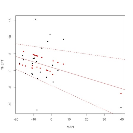
The black dots are the observed data, the red dots are the fitted mu[i] values from the JAGS run. Notice “shrinkage” towards the mean. This so-called “borrowing of strength” is a feature of Bayesian analysis. The solid red line is the regression from the model. The dashed lines are upper and lower limits based on regressions of the 2.5% and 97.5% probability limits on the fitted values.
Perhaps most importantly, though, notice the outlying variable that is likely responsible for pulling the overall results toward significance. It is the data from the 20th precinct on the west side of Midtown Manhattan, where there was an experimental 40% increase in manpower during the experimental period. Two quick take home messages are (1) plotting data is usually more informative than summary statistics, and (2) substance area knowledge is essential to correctly interpret any kind of analysis.
We could take a couple of approaches to this outlier. We could delete the data point, but throwing out data is usually not a good idea. Or we could attempt to make our analysis more robust to outliers. Bayes makes this relatively painless, by allowing us to specify the model with more robust t-distributed errors.
1 2 3 4 5 6 7 8 9 10 11 12 13 14 | cat( "model{ for (i in 1:23) { THEFT[i] ~dt(mu[i] , tau, 4) # robust likelihood t on 4 df mu[i] <- beta0 + beta1*MAN[i] + beta2*DIST2[i] + beta3*DIST3[i] } beta0 ~dnorm(0, 0.00001) beta1 ~dnorm(0, 0.00001) beta2 ~dnorm(0, 0.00001) beta3 ~dnorm(0, 0.00001) tau ~ dgamma (0.001, 0.001) sigma2 <- 1/tau}", file="m2.jag" ) |
You will find that in this instance the results do not change too very much (we may want to consider an even more robust distribution like a double exponential), but it does illustrate the relative ease with which you can update models.
Logistic Regression
Logistic models are among the most popular multivariable approaches to the often dichotomous outcomes addressed by epidemiology. Fortunately, Bayesian model specification is fairly straightforward regardless of the type of regression. As an example of logistic regression in the Bayesian setting, we look at myocardial infarction in hospitalized patients. The data come from the US National Heart Lung and Blood Institute and are based on a 1997 study of the digitalis. The data set dig2 contains a random sample of 2000 observations from the original data set. The outcome variable is myocardial infarction (“MI”) coded as 0 or 1, and variables for age, gender and body mass index.
We begin by specifying a model. The process is similar to that for a linear model. We set up a loop over each observation, but here specify the likelihood as a Bernoulli-distributed outcome (rather than normally distributed) with the parameter “mu” explicitly defined as a logistic model. This model should look familiar from your statistics training, and you may be beginning to appreciate how syntactic modeling, of which BUGS and JAGS is an example, differs from some popular statistical software like SAS. After specifying the likelihood, we specify prior distributions for the \(\beta\) coefficients. Here we apply only vaguely informative normal distributions to allow the data to “speak for themselves”. In a later session we’ll discuss a bit more about choosing priors for Bayesian models.
1 2 3 4 5 6 7 8 9 10 11 12 | cat( "model { for( i in 1 : N ) { MI[i] ~ dbern(mu[i]) mu[i]<-1/(1+exp(-(b0 + b1*AGE[i] + b2*SEX[i] + b3*BMI[i]))) } b0 ~ dnorm( 0 , 1.0E-12 ) b1 ~ dnorm( 0 , 1.0E-12 ) b2 ~ dnorm( 0 , 1.0E-12 ) b3 ~ dnorm( 0 , 1.0E-12 ) }", file="logistic.jag" ) |
Note that we could, equivalently, have specified the model as:
MI[i] ~ dbern(p[i])
logit(p[i]) <- b0 + b1*AGE[i] + b2*SEX[i] + b3*BMI[i]
Next, we read in the data set and define the data structure for the JAGS run. Note, we are including the number of rows for the variable “N” in our model statement.
1 2 3 | mi<-read.csv("/Users/charlie/Desktop/dig2.csv",header=T, stringsAsFactors=F) dat1<-list(MI=mi$MI, AGE=mi$AGE, SEX=mi$SEX, BMI=mi$BMI, N=nrow(mi)) |
In setting up our initial values we take a different approach than we did before. As noted in the section describing the machinery of MCMC, starting or initial values can have an effect on how efficiently the algorithm covers the sample space. There are no hard and fast rules for choosing initial values beyond the recommendation that they be “realistic” (so the MCMC sampler will run efficiently) and “over-dispersed” (so we can better assess convergence to a stable posterior distribution). One approach (that appeals to me) is to set the choice of initial values on a simple MLE run of the model. This has the added benefit of allowing you to compare your Bayesian results to those of a frequentist approach. Here, we extract the coefficients from a GLM logistic model (to get “realistic” values) and add / subtract a hopefully reasonable number (to “disperse” the initial values). The structure for the data object holding the initial values is a list of lists.
1 2 3 4 5 6 7 8 9 | estInits<-with(mi, glm(MI~AGE+SEX+BMI, family=binomial(logit))) estInits inits<-list( list(b0=estInits$coef[1]+.5, b1=estInits$coef[2]+.1, b2=estInits$coef[3]+.1,b3=estInits$coef[4]+.1), list(b0=estInits$coef[1]-.5, b1=estInits$coef[2]-.1, b2=estInits$coef[3]-.1,b3=estInits$coef[4]-.1) ) |
Next, define the parameters we want to monitor, run the JAGS program and take a quick look at the results.
1 2 3 4 5 6 7 8 9 10 11 12 13 14 | parameters<-c("b0", "b1", "b2", "b3") library(R2jags) logmod<- jags(data = dat1, inits = inits, parameters.to.save = parameters, model.file = "logistic.jag", n.chains = 2, n.iter = 5000, n.burnin = 2000, n.thin = 1) logmod |
The point estimates are very close to those of the GLM run. This is expected. When you have a lot of data (and 2000 observations is a decent number) and very vague or only minimally informative priors, the likelihood predominates and you get the MLE estimates. You still, of course, have the benefits of being able to make direct probability assessments of your results, which are not available from a strict MLE frequentist model, and you can do things like update your results, add observations, calculate probabilities for complex functions etc…
You will notice that the model takes appreciably (depending on your machine, perhaps annoyingly) longer to run. This could be a function of the model itself. Simon Jackman recommends grouping binary or Bernoulli-distributed data into Binomial data to improve model behavior. But, in general, long model run times is a drawback of Bayesian analysis, especially with larger data sets. Some folks complain about having to run their simulations overnight to get reasonable estimates. If you have a model that seems to take inordinately long to run, take a close look at the convergence diagnostics (which you should do anyway…) Let’s take a quick look at the traceplots.
1 | plot(as.mcmc(logmod)) |
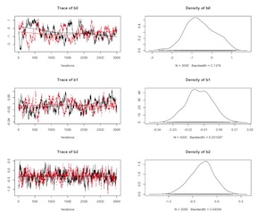
Logistic Model Un-Centered Covariates
The convergence for nodes b1 and b3 is problematic. As we’ve discussed above, one approach to this issue is to center or standardize the data. Here, let’s mean center the problematic variables and re-run the model.
1 2 3 4 5 6 7 8 9 10 11 12 13 14 | dat1<-list(MI=mi$MI, AGE=(mi$AGE-mean(mi$AGE)), SEX=mi$SEX, BMI=(mi$BMI-mean(mi$BMI)), N= |
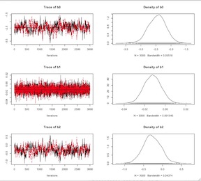
Logistic Model Centered Covariates
The model should run faster. The trace plots should indicate appreciably better convergence. Finally here is a little code for extracting the (exponentiated) point estimates and a second line of code for extracting the (again exponentiated) point estimates with their 95% credible intervals. Clearly, the variable are not vary predictive of myocardial infarction in this population.
1 2 | lapply(logmod$BUGSoutput$mean, FUN=exp) exp(logmod$BUGSoutput$summary[,c(1,3,7)]) |
Other Models
There are many other potential approaches to single-level Bayesian modeling. I have a write up on Poisson models in the setting of spatial analysis here. Perhaps the most comprehensive freely available source of models is the WinBUGS User Manual. If you are interested in non-linear regression models, I recommend the “Dugongs” example.
Categorical Outcomes
For categorical outcomes you can use the “dcat” distribution:
y[i]~dcat(p[ ])
Where p[ ] is an array of probabilities.
As an example of how you might use this distribution, imagine you are told a fair coin came up head 10 times and you want to model how many times it was tossed, i.e. you want to make inferences on the denominator “n” of a binomial distributed variable.
You could paste the following code directly into a WinBUGS or OpenBUGS window and run it:
model{
r <-10
q <- 0.5
r ~dbin(q, n)
n.cont ~ dunif (1, 100)
n <- round (n.cont)
}
It should return a median value of 21, with a 95% probability that the true number of tosses is somewhere between 13 and 32. But this approach is actually something of a hack. We are placing a continuous uniform prior on the discrete variable “n” and making use of the round() function to return a discrete result.
We could, though, put a discrete uniform prior on “n” by using the “dcat” distribution as follows:
model{
r <-10
q <- 0.5
r ~dbin(q, n)
  # discrete prior on 10 to 100
for (j in 1 :9)  {  p[j] <-0  }
for (j in 10:100)  {  p[j] <- 1/91}
n ~ dcat (p[])
}
We should get the same answer.
Multinomial Outcomes
The multinomial distribution is a useful extension of the binomial. Rather than a single probability for all outcomes, each outcome has its own probability. Suppose you have an outcome variable that is an array of 3 counts in K categories, e.g. y = (1,2,4), (3,3,3), etc… You can model these data with a multinomial distribution:
for (i in 1:N) {
  y [i, 1:3] ~ dmulti(q[], n[i])   # multinom distro vector responses
  n[i] <- sum(y[i, ])
}
If there are no covariates, you can place a Dirichlet Prior on q[ ] so that \(Pr(q) \propto q_k^\alpha\) :
q[1:3] ~ ddirch(alpha [])
\(\alpha\) needs to be a fixed quantity e.g.:
for (k in 1:3)  {
      alpha[k] <- 1
}
returns a uniform prior on q.
Note that you need to specify the dimension of vectors or arrays on the left hand side of distributions in the BUGS language e.g. 1:3 tells BUGS how much space to allocate.
If you have covariates, you can use a multinomial logistic model, which is equivalent to K-1 logistic regressions comparing k > 1 with category 1, the details of which can be found here.
Hierarchical Models
Introduction
Say, as we so often do in probability, you are flipping coins.6 But now, rather than just being interested in the coins themselves, you are also interested in the mints from which they came. So, there are two parameters, the behavior of the coins themselves and the influence of the factory in which they were minted. We may believe that the two parameters are independent, e.g. whether a coin lands heads or tails has nothing to do with the mint from which it came. In which case, you could look at the results of all the coin tosses as a single large experiment. Or, we may believe that the two parameters are somehow related, e.g. the factory in which a coin was minted may influence whether it turns up head or tails.
In Bayesian modeling, parameters that affect data directly are termed, well, parameters. Parameters that affect data indirectly or through other parameters, like the factory in which a coin was minted, are termed hyperparameters. From the practical perspective of conducting Bayesian analysis, they are essentially treated the same, i.e. they are both part of the joint multidimensional parameter space to which we apply Bayes’ rule to update our prior beliefs to some posterior distribution. They clearly, though, have substantive importance in interpreting our analysis. And, given the complexity of the relationships, they will more frequently require Gibbs rather than Metropolis sampling algorithms.
Returning to our coin and factory hierarchy, we begin by specifying a binomial likelihood for the toss of a coin: \(\sum p^x *q^{{n-x}}\), where \(p=\theta\) and \(q=1-\theta\). We can place a \(Beta(a,b)\) prior on this likelihood: \(p(\theta) \sim Beta(\alpha,\beta)\)
Now, for the hierarchical part. Instead of specifying a single value for \(\alpha\) and another value for \(\beta\), the parameters that define our prior, we allow them to vary according to some probability distribution. We could, for example, think of \(\alpha\) and \(\beta\) taking on any value between 0 and 1 and place a uniform prior on them in our model specification: \(p(\alpha) \sim Unif(0,1)\) and \(p(\beta) \sim Unif(0,1)\) . The model is hierarchical because there are two levels of uncertainty. The first is represented by the \(Beta(\alpha,\beta)\) prior on \(\theta\). The second layer of uncertainty is the prior on the effect of \(\alpha\) and \(\beta\) on the Beta prior. If we were certain about \(\theta\), or had a lot of data about \(\theta\), the layers of the model could collapse to single values for \(\alpha\) and \(\beta\). In general, you will find Bayesian hierarchical models characterized by two levels of uncertainty for parameters of interest. Also note, that the models are inherently nested, with one level of uncertainty nested in another.
About shrinkage and outliers
If the behavior of the coins (\(\theta\)) depends in part on the shared influence of the mint in which they were created, then the bias in an individual coin is related to the bias in other coins from the same mint. If the outcomes for the coins are similar, then, the posterior distribution for the dependence of \(\theta\) on \(\alpha\) and \(\beta\) will have a high mean value, and individual results will more closely resemble \(\theta\). This “shrinkage” of individual measurements will be most evident in outliers, which will be pulled closer to the behavior of the other coins, than the other coins will be pulled toward the outlier.
Approach to Bayesian Hierarchical Models in BUGS and JAGS
In hierarchical models (also referred to as ‘mixed’ or ‘multi-level’ models) you are generally interested in making inferences on many parameters \(\theta_1\) … \(\theta_i\) measured on N ‘units’ (individuals, subsets, areas, time-points, trials etc…) which are related in some way.
We can make 3 possible assumptions about the \(\theta\)’s:
- the \(\theta\)’s are identical, in which case all the data can be pooled and the units from which the data arose can be ignored
- the \(\theta\)’s are independent and entirely unrelated, in which case each unit from with the data arose should be analyzed separately
- the \(\theta\)‘s are exchangeable or similar which is a compromise between independent and identical relationships. From the Bayesian perspective, rather than applying a prior to the individual measurements distributed across the entire sample (identical \(\theta\)’s) or a separately applied prior for each (independent) \(\theta\)’, we assume the individual measurements vary within each unit, and across units.
Example: Hierarchical Model for THM Concentrations
Recall the conjugate normal-normal model from section 1 of these notes where we estimated the mean THM concentration from two measurements in a zone. Say now we had a full data set of THM measurements for 70 water supply zones with multiple measurements in each zone with not all zones having the same number of measurements. We can assume a normal likelihood for the data in each zone:
\(x_{iz} \sim N(\theta_z, \sigma^2_z)\) for i=1…\(n_z\), z=1-70
Note that the likelihood now specifies 70 parameters (\(\theta_z\)) for the mean THM concentration.
If we assume a that \(\theta_z\) are are the same for each zone (identical parameters) we specify a single prior, e.g \(\theta \sim N(\mu , \sigma^2)\). If it doesn’t make sense to expect zones supplied by different water sources to have identical THM levels (and it probably doesn’t), we can take another approach. We might assume that each zone is essentially an independent experiment in measuring THM concentrations and the results in one zone are entirely unrelated to results in any other zone. In this case, we could specify an explicit prior for each \(\theta\) for 70 descriptive studies. But do we really believe that knowing, say, the results for 69 zones tells us absolutely nothing about the results for the remaining 70th zone? If we believe there is likely some room for “pooling” or “borrowing” information across zones to smooth our estimates, we may assume exchangeability across zones. In addition to a prior distribution for each \(\theta\), we might very well believe there is an appropriate prior for how the \(\theta\)’s themselves vary.
Rather than specify an independent prior for each \(\theta\), we could specify a hierarchical prior: \(\theta_z \sim N(\mu, \sigma^2z_{[z]})\) where \(\mu\) and \(sigma^2z_{[z]}\) are unknown parameters for how the \(\theta\)’s vary and are to be estimated. (The [ ] nomenclature indicates labels for each zone or unit from which the observations arise, not the individual observations themselves). We then assign prior distributions to the hyperparameters:
\(\mu \sim N(0,100000)\) \ \(sigma^2z_{[z]} \sim Gamma(0.001, 0.001)\) (a joint prior distribution for the entire set of parameters)
The formulas for the full joint prior distribution (at both levels of specification) and the joint posterior are complex, but with BUGS we only have to specify the local relationships, and the Bayesian MCMC machinery proceeds as usual to simultaneously estimate the joint posterior distribution for all the unknown quantities. The posterior for each \(\theta_z\) “borrows strength” from the likelihood contributions of all the zones through the joint influence of the priors for the hyperparameters. This leads to a global smoothing of the THM levels for each zone, and reflects our uncertainty about he true values of the hyperparameters.
Here is a graphical representation (taken from David Spiegelhalter’s Cambridge WinBUGS course) of the three approaches to the THM data:
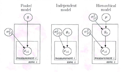
Where
- \(\theta_z\) is the mean THM concentration for zone z for the study period
- \(\mu\) is the overall mean THM concentration across all zones for the study period
- \(\sigma^2_{[z]}\) is the between zone variance in THM concentrations
- \(\sigma^2_{[e]}\) is the residual variance in THM concentrations (reflects measurement error and true within zone variation in THM levels)
And here is a graphical illustration (also from Dr. Spiegelhalter) of the global smoothing of the hierarchical estimates:
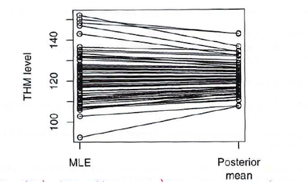
BigBayes11
The model specification is not limited to globally-smoothed estimates. You can have locally smoothed estimates by specifying a zone-specific error variance \(\sigma^2_{[e]z}\) for each measurement and placing a prior on it. Or you could use specify a conditional autoregression (CAR) model with weights based on whether zones neighbor each other (see my notes on Bayesian approaches to spatial data). These kinds of locally smoothed estimates may be difficult or impossible with non-BUGS approaches.
A couple of notes of caution are in order. First, smoothing is appropriate when you feel the variation in the raw numbers exceeds what is actually going on, e.g. over-dispersion in a Poisson model. But, you don’t want to smooth away something that is actually causing the variation in the raw numbers, e.g. a cluster or “hot spot” in your data. In that case, you might include a term to account for the variation. Second, if there is missing data, you will not get results for those units on the raw scale. The hierarchical model will return results for those units.
Coding the Model
The THM data are “ragged” in that they there are unequal numbers of observations for each zone. We can code these data in one of three ways: (1) using offsets, (2) with a nested index, or (3) padding out the entries with NA’s.
The offset variable tells BUGS where each zone’s measurements begin and end, e.g. zone 1 starts at 1 and has 4 observations, zone 2 begins at 5 and has 6 observations etc.
In the model statement, you identify the zones as part of the likelihood, and then place priors on the random effects mean and variance.
1 2 3 4 5 6 7 8 9 10 11 12 13 | cat("model{for (z in 1:Nzone){ for(i in offset[z]: (offset[z+1]-1)) { thm[i] ~ dnorm(theta[z], tau.e) # likelihood } theta [z] ~dnorm(u, tau.z) # zone mean (random effects) mu ~ dnorm(0, 0.000001) tau.z ~ dgamma(0.001, 0.001) sigma2.z <- 1/tau.z # random effects variance tau.e ~ dgamma(0.001, 0.001) sigma2.e <- 1/tau.e # residual error variance}", file="thm1.jag") |
Then you set up your data to reflect the structure in the model:
Data
1 2 3 4 | dat1<-list(Nzone=70, thm=c(111.3, 112.9, 112.9, 105,5, 122.6 etc…), offset= c(1, 5, 11, etc….) ) |
Using a nested index is more computationally efficient. In this neater approach, each observation is keyed to a zone.
1 2 3 4 5 6 7 8 9 10 11 12 13 14 15 16 | cat("model{for(i in 1:Nobs) { thm[i] ~ dnorm(theta[zone[i]], tau.e) # likelihood } for(z in 1:Nzone) { theta[z] ~ dnorm(mu, tau.z) # zone means (random effects) } # priors mu ~ dnorm(0, 0.000001) tau.z ~ dgamma(0.001, 0.001) sigma2.z <- 1/tau.z # betw-zone (random) var of mean THM) tau.e ~ dgamma(0.001, 0.001) sigma2.e <- 1/tau.e # residual error variance }", file="thm2.txt") |
And a data statement to, again, reflect the structure in the model.
1 2 3 | dat2<-list (Nobs=173, Nzone = 70, thm = c(111.3, 112.9, 112.9, etc…), zone = c(1, 1, 1, 1, 2, 2, 2, 2, etc…) |
Finally, you could “pad out” the observations with NA’s. Basically, this makes the data list balanced and rectangular. It is easier, perhaps, to write the model code, but it is computationally clumsier in that it causes BUGS or JAGS to spend a lot of time doing useless calculations on the NA’s.
The Variance Partition Coefficient (aka Intraclass Correlation)
The Variance Partition Coefficient or Intraclass Correlation is the between group variance divided by the sum of the between group variance plus within group variance. In hierarchical or multilevel models, the residual variation in the response variable is split into components attributed to different levels. This is a defining characteristic of so-called random effects models, whether Bayesian or frequentist. Essentially, you are partitioning the error component of the model into that which can be accounted for by the variation among the units from which the observations arise (the “random effects” component), and the remaining unstructured error. You may be interested in quantifying the percentage of the total variation attributable to higher level units, or the proportion of variation due to the random effects component.
In a 2-level normal, linear model, you can calculate:
\[ VPC=\frac{\sigma^2_{[e]}}{\sigma^2_{[z]}+\sigma^2_{[e]}} \]
Where, \(\sigma^2_{[e]}\) is the first level Normal likelihood variance \(\sigma^2_{[z]}\) is the second level random effects variance
To code for this in BUGS or JAGS, simply add a line of code to your model:
vpc <- sigma2.z / (sigma2.z + sigma2.e)
Then monitor “vpc” as a node. So for example, in the THM data, the posterior mean for the VPC is 0.49 with a 95% credible interval of 0.32 to 0.64, indicating that about half the variance in the data was due to between zone variation.
Your turn…
Take a moment to try to fit this model in JAGS using R2jags. You can find the data here. Use the model statement above; add the line of code to calculate the variance partition coefficient. Monitor the mean, the variances and the variance partition coefficient. To keep things simple, let JAGS provide initial values for this (to do this, just omit the initial values statement in the R2jags model run.) If you need it, the full syntax is here
Example: Hepatitis B Immunization in Africa
Hepatitis B is endemic in Africa. A national vaccination program was introduced in the Gambia. The program effectiveness depends on the duration of immunity. In a study of program effectiveness, 106 children were immunized. Baseline titers were drawn at the time of vaccination, and 2 or three times afterward. Investigators were interested in developing a useful model for predicting a child’d protection against hepatitis B after vaccination. A similar study in Senegal found titer levels were proportionate to the inverse of the time since vaccination, \(titer \propto 1/t\).
As the following figure indicates, the data are very messy.
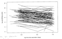
As a first approach, we might specify a non-hierarchical linear model,
\[ y_{ij} \sim N(\mu_{ij}, \sigma^2) \],
where \(y_{ij}\) is the log of the \(j^{th}\) titer for the \(i^{th}\) child. A linear predictor could be
\[ \mu_{ij} = \beta_0 \beta_1 * (t_{ij} - \bar{t} + \beta_3 * (y_{0i} - \bar{y_0})) \],
where \(t_{ij}\) is the log time of days since the \(j^{th}\) vaccination for child \(i\), and \(y_{0i}\) is the log baseline titer for child \(i\).
The problem with this approach is that it assumes a common regression line for all the children and takes no account of the repeated measurements within children. To address these issues, we can take a hierarchical approach to a linear mixed or random coefficients model where we modify the linear model to allow separate intercepts and slopes for each child:
\[ \mu_{ij} = \beta_{0i} \beta_{1i}* (t_{ij} - \bar{t} + \beta_3 * (y_{0i} - \bar{y_0})) \],
Note the subtle but important difference from the linear model in this specification. Now there is a separate intercept (\(\beta_{0i}\)) and slope (\(\beta_{1i}\)) for each child. This is analogous to the THM example, but instead of “zones” we have multiple measurements on each child. Similarly, we assume that the intercepts (\(\beta_{0i}\)) and slopes (\(\beta_{1i}\)) are “exchangeable”. In our Bayesian model specification, we now place priors on both parameters,
\[ \beta_{0i} \sim N(\mu_{\beta 0}, \sigma^2) \\ \beta_{1i} \sim N(\mu_{\beta 1}, \sigma^2) \\ \]
And place \(N(0, .00001)\) hyperparameters on \(\mu_{\beta 0}\) and \(\mu_{\beta 1}\)
Despite the complexity of the model, the implementation in BUGS or JAGS only involves specifying local relationships and proceeds in a familiar fashion. We are again faced with ragged data of 2 or 3 observations per child. A nested index formation would look like this:
1 2 3 4 5 6 7 8 9 | ("model{for (k in 1:TotalObs) { y[k] ~ dnorm(mu[k], tau) mu[k] <- alpha[child[k]] + beta[child[k]] * (t[k]-tbar) + gamma*(y0[child[k]] – y0bar) } For (i in 1:N) { alpha[i] ~ dorm(mu.alpha, tau.alpha) beta[i] ~ dnorm(mu.beta, tau.alpha) }}", file= "hepb.jags") |
And the data specification to reflect the model structure looks like this:
1 2 3 4 5 | dat<-list (N=106, TotalObs=288, y = c(4.99, 8.02, 6.83, 4.91, etc...), t = c(6,54, 6.96, 5.84, 6.52, etc...), child = c(1,1,2,2, etc...), y0 = c(8.61, 8.61, 7.10, 7.10, etc...) |
Your turn…
I was fortunate enough to track down the original data in a WinBUGS archive email from Dr. David Spiegelhalter. Try coding and running the model in JAGS. This time, though, try using the “offset” approach I described in the THM example. Again, for simplicity sake, allow JAGS to supply the initial values. If you need it, the answer is here
Additional levels of hierarchy
It is (relatively) straightforward to extend the linear approach to generalized models (Poisson, Logit), and to incorporate additional levels of hierarchy or uncertainty, e.g. measurements within zone, within regions, with cross-classified hierarchies. Here is some model code an example of a (somewhat) more complicated model with an additional level of variation. The code was written for a data set of 800 observations on children who attended 132 primary and 19 secondary schools in Scotland. (They came originally from a training data set for the “MLWin” software package) The variables are:
- Y = exam attainment score at age 16
- VRQ = verbal reasoning score taken on secondary school entry
- SEX = gender (0=boy, 1=girl)
- PID = primary school ID code
- SID = secondary school ID code
The following code is for a normal hierarchical model with independent random effects for primary school and secondary school. Gender and verbal reasoning included as ‘fixed’ covariate effects (although since Bayesian, these ‘fixed’ effects still assigned prior distributions).
for (i in 1:Nobs) {
  Y[i] ~ dnorm(mu[i], tau.e)
  mu[i] <- alpha + beta[1]*SEX[i] + beta[2]*VRQ[i] + theta.ps[PID[i]] + theta.ss[SID[i]]

}

 # random effects distributions (note: non-centered)
for (j in 1:Nprim) { theta.ps[j] ~ dnorm(0, tau.ps) } # primary school effects
for (k in 1:Nsec)  [ theta.ss[k] ~ dnorm(0, tau.ss } secondary school effects

 # priors on regression coefficients and variances
tau.e ~ dgamma(0.001, 0.001) # residual error variance
sigma2.e <- 1/tau.e
tau.ps ~ dgamma(0.001, 0.001) # between primary school variance
sigma2.ps <- 1/tau.ps
tau.ss ~ dgamma(0.001, 0.001) # between secondary school variance
sigma2.ps <- 1/tau.ps
alpha ~ dnorm (0, 0.00001) # intercept
for (q in 1:2) { beta[q] ~ dnorm 0.00001 } # regression coefficients

 # percentage variance of total variance explained...
VPS.ps <- sigma2.ps / (sigma2.3 + sigma2.ps + sigma2.ss) #...by primary school

VPS.ps <- sigma2.ss / (sigma2.3 + sigma2.ps + sigma2.ss) #...by secondary school
Example: The Western Australia Pregnancy (Raine) Cohort Study
The Raine Cohort started as an RCT of potential adverse effects of ultrasound. All subjects were given routine US at 18 weeks. Then randomized to additional US at 24, 28, 34, and 38 weeks. The project was subsequently converted to a cohort study. Because the data quantified fetal growth with serial biometric data, the study was used to investigate the so-called “fetal origins” hypothesis that fetal adaptation to an adverse intrauterine environment results in permanent physiological changes. (Prenatal ultrasound biometry related to subsequent blood pressure in childhood. K Blake, L Gurrin, et al. J Epidemiol Community Health. 2002 September; 56(9): 713–718.) Researchers investigated whether there was an inverse relationship between low birth weight and subsequent hypertension.
The data consisted of 3450 ultrasound exams for 5 fetal dimensions on 707 fetuses. We will just consider head circumference, where \({Y}_{ij}\) is the measured head circumference for the \({i}^{th}\) fetus at the \({j}^{th}\) timepoint \({t}_{ij} = 18, 24, 28, 34, 38\) weeks.The number of measurements for a fetus varied between 1 and 7. (As part of their analyses, the researchers transformed (Box-Cox) the data to establish a linear relationship, but that need not concern us here.)
A , based on an assumption of complete homogeneity, would have a single fixed intercept and a single fixed slope for all the data: \({y}_{ij} = {\beta}_{0} + {\beta}_{1} * {x}_{ij} + {\varepsilon}_{ij}\), where \({\varepsilon}_{ij} \sim N(0,{\sigma}_{\varepsilon}^{2})\)
By now, you should be thinking that the repeated measures in this longitudinal data set suggest a hierarchical or linear mixed model, 7 with subject-level (repeated measures) intercepts and slopes:
\[ {Y}_{ij} = ({\beta}_{0} + {u}_{0i}) + ({\beta}_{1} + {u}_{1i}){X}_{ij} + {\varepsilon}_{ij}, \]
Where, for the \(j^th\) measurement on the \(i^th\) fetus (\(i=700\)),
- \(\beta_0\) is the fixed intercept for each child
- \(u_{0i}\) is the random intercept for each child
- \(\beta_1\) is the fixed slope for each child
- \(u_{1i}\) is the random slope for each child
The model follows a bivariate normal distribution
\[ \begin{equation*} \left({\begin{array}{c} {u}_{0i} \\ {u}_{1i} \end{array}}\right) = {\text {N}}_{\text {2}} \left[{\left({\begin{array}{c} 0 \\ 0 \end{array}}\right),\left[{\begin{array}{cc} {\sigma}_{0}^{2} & {\sigma}_{01} \\ {\sigma}_{01} & {\sigma}_{1}^{2} \end{array}}\right]}\right] \end{equation*} \]
where \(\sigma_{1}^{2}\) allows for covariance between the slope and the intercept while centering the model.
In the following code. I step through the analyses for these data.
Fitting the Model
We begin, as we should, by looking at the data. Start by reading and exploring the Raine data. There are variables for id, head circumference and gestational age. We are interested in the relationship between head circumference and gestational age. The variable “tga” is the transformed gestational age (\(tga = ga − 0.0116638 * ga^2\)) which makes the relationship between head circumference and gestational age linear.
1 2 3 | fetal <- read.csv(".../fetal.csv",header=TRUE) str( fetal) # id, head circumference, gestational age, head( fetal, 10 ) |
We tabulate the number of measurement for each child, and see that the majority of children had 4 or 5 repeated measures, but they range from 1 to 7. We then create so-called “spaghetti plots” for a random sample of 100 of the 706 fetuses, demonstrating the linearizing effect of the transformation, and that the square root transformation of head circumference makes the relationship between it and gestational age more linear.
1 2 3 4 5 6 7 8 9 10 | with(fetal, addmargins(table(table(id)))) # tab number measurements per kid par( mfrow=c(1,3), mar=c(3,3,1,1), mgp=c(3,1,0)/1.6 ) id.sub <- sample( unique(fetal$id), 50 ) with( fetal, plot( ga, hc, type="n" ) ) for( i in id.sub ) with( subset(fetal,id==i), lines(ga,hc) ) with( fetal, plot( tga, hc, type="n" ) ) for( i in id.sub ) with( subset(fetal,id==i), lines(tga,hc) ) with( fetal, plot( tga, sqrt(hc), type="n" ) ) for( i in id.sub ) with( subset(fetal,id==i), lines(tga,sqrt(hc)) ) |
Before moving on to a hierarchical Bayesian model in JAGS, let’s (again, as we should) take a more straightforward approach and fit a model using the R package “lmer4”, which despite our interest here in Bayesian modeling is the R tool of choice mixed models. 8
In “mler4” models are specified with fixed (not varying by group) and random (varying by group) variables:
1 | lmer (y ~ fixed + (1 + random | group)) |
The number 1 is used to specify that the intercept varies by group, the term “random” stands in for a variable with varying slope. You can also use it to specify GLM models:
1 2 | lmer (y ~ fixed + (random | group), family=binomial (link=“logistic”)) |
We fit a random effects linear model for an outcome measure of (fetus “f” at time “t”) square root of head circumference \(y_{ft}\) for each fetus at time t. For simplicity in this illustrative model, we’ll specify that each child’s measurements across time (slopes) are parallel to each other, but vary by intercept. The \(\beta_0\) intercept is not really interpretable in this contect (no child has a head circumference of 0), and we could if we wanted set it to some baseline level, e.g. at age 18 months by centering the gestational age variable (I|tga-18). The \(\beta_1\) coefficient reflects the (fixed) effect of time. The random effect is, again, that the intercept is allowed to vary for each child relative to each other (1 | id) though (again) the slopes are otherwise parallel to each other.
1 2 3 4 5 | library( lme4 ) m0 <- lmer(sqrt(hc) ~ tga + (1 | id), data=fetal) summary(m0) fixef(m0) VarCorr(m0) |
In the summary statistics, we see the intercept is estimated as -.08 but (as noted above) is not really interpretable here. The effect of time is the tga estimate of 0.086 or about a 1 cm increase in head circumference per week. The random effects result of interest is “id (Intercept) 0.059714 0.24437” which tells us that each child’s series of results (the regression line) varies from each other by about 0.24 cm. The residual result “Residual 0.062665 0.25033” is interpreted as usual, i.e. it is the difference between the observations and the predictions (from the regression line). We can extract estimates and variances with fixef(m0) returning the same results as the summary shows. We request a variance-covariance matrix for the random effects with VarCorr(m0), which is not very informative for this very simple model, since there is only one random effect term and it correlates with itself as 1.
Now let’s fit a Bayesian model of the same data in JAGS. In this run, we’ll model the untransformed head circumference as an outcome, and the mean-centered time (tga) variable as a fixed effect. (As a comparison, try doing this with lmer() …) In the model statement the random effect for each child is represented as sigma.u, the error as sigma.e
1 2 3 4 5 6 7 8 9 10 11 12 13 14 15 16 17 18 19 20 21 22 23 24 25 26 27 28 | cat(" model { for( j in 1:N ) # for each observational unit { mu[j] <- beta[1] + beta[2] * ( tga[j]-18 ) + u[id[j]] hc[j] ~ dnorm( mu[j], tau.e ) } for( i in 1:I ) # random effects for each person { u[i] ~ dnorm(0,tau.u) } # Priors: # Fixed intercept and slope beta[1] ~ dnorm(0.0,1.0E-5) beta[2] ~ dnorm(0.0,1.0E-5) # Residual variance tau.e <- pow(sigma.e,-2) sigma.e ~ dunif(0,100) # Between-person variation tau.u <- pow(sigma.u,-2) sigma.u ~ dunif(0,100) }", file="fetalJags1.txt" ) |
Next, we define the data elements, including defining the N observations over I individuals, and use the attr() function to extract initial values form our lmer run.
1 2 3 4 5 6 7 8 9 10 11 12 13 14 15 16 17 18 19 20 21 22 23 | fetal.dat <- list( id = as.integer( factor(fetal$id) ), hc = fetal$hc, tga = fetal$tga, N = nrow(fetal), I = length( unique(fetal$id) ) ) ( sigma.e <- attr(VarCorr(m0),"sc") ) ( sigma.u <- attr(VarCorr(m0)$id,"stddev") ) ( beta <- fixef( m0 ) ) fetal.inits <- list( list( sigma.e = sigma.e/3, sigma.u = sigma.u/3, beta = beta /3 ), list( sigma.e = sigma.e*3, sigma.u = sigma.u*3, beta = beta *3 ), list( sigma.e = sigma.e/3, sigma.u = sigma.u*3, beta = beta /3 ), list( sigma.e = sigma.e*3, sigma.u = sigma.u/3, beta = beta *3 ) ) |
And now set the parameters we want to monitor, run the model in JAGS, and explore the results.
fetal.params<-c(“beta”, “sigma.e”, “sigma.u”)
1 2 3 4 5 6 7 8 9 10 11 12 13 14 15 | library(R2jags) jag.fetal<-jags(data=fetal.dat, inits=fetal.inits, parameters.to.save=fetal.params, n.chains=4, n.iter=500, n.thin=20, model.file="fetalJags1.txt") jag.fetal summary(jag.fetal) print(jag.fetal) plot(jag.fetal) traceplot(jag.fetal) jag.mcmc.fetal<-as.mcmc(jag.fetal) plot(jag.mcmc.fetal) |
The results will differ from the lmer run because the BUGS model has untransformed head circumference as a dependent, and the bugs model has the transformed gestational age adjusted to the 18th week (tga[j]-18).
To fit a (likely) more realistic model with both random intercept and slope, we need only alter the code slightly. First, in lmer4.
1 2 3 4 5 | library(lme4) m0 <- lmer(hc ~ tga + (1 + tga | id), data=fetal) summary(m0) VarCorr(m0) |
We see a strong (~0.9) correlation between the random components, indicating that fetuses with the smallest head circumferences at baseline have steeper slopes in the regression line. Again, some simple centering helps address this issue, and when we update the model, we see less correlation. For good measure, we take a look at a qqplot to assess the normality of the residuals.
1 2 3 4 5 6 7 8 9 | fetal <- transform(fetal, tga.cent=tga-18) m1 <- lmer(hc ~ tga.cent + (1 + tga.cent | id), data=fetal) summary(m1) VarCorr(m1) m1.res<-residuals(m1) qqnorm(m1.res) # check normality of residuals |
Now, let’s model it in JAGS. It is a good deal more complex than the approach in lmer4. 9
When specifying the model, we first fix the data elements to be used in the model definition, then define the model. Note that in defining our priors, we also have to define a prior for the variance-covariance matrix of the random effects. The Wishart prior for the for random effect variance-covariance takes takes a 2x2 matrix as input, with R as a mean value, defined at the beginning or model statement. Note that the two values are in two different scales, cm for head circumference, and change in head circumference per week.
1 2 3 4 5 6 7 8 9 10 11 12 13 14 15 16 17 18 19 20 21 22 23 24 25 26 27 28 29 30 31 32 33 34 35 36 37 38 39 40 41 | cat(" # fixing data to be used in model definition data { zero[1] <- 0 zero[2] <- 0 R[1,1] <- 0.1 R[1,2] <- 0 R[2,1] <- 0 R[2,2] <- 0.5 } model { for( i in 1:I ) # intercept and slope ith kid, incl random effects { u[i,1:2] ~ dmnorm(zero,Omega.u) # biv nl (2 r.e.'s, (intercept, slope) q fetus } # Define model for each (jth) observation or measurement for( j in 1:N ) { mu[j] <- ( beta[1] + u[id[j],1] ) + ( beta[2] + u[id[j],2] ) * (tga[j]-18 ) hc[j] ~ dnorm(mu[j], tau.e) } # Priors: # Fixed intercept and slope beta[1] ~ dnorm(0.0,1.0E-5) beta[2] ~ dnorm(0.0,1.0E-5) # Residual variance tau.e <- pow(sigma.e,-2) sigma.e ~ dunif(0,100) # variance-covariance matrix of the random effects sigma.u <- inverse(Omega.u) Omega.u ~ dwish( R, 2 ) } file="fetalJags2.txt") |
In defining the data, the grouping variable has to be a factor, and even if it is a factor in the data, it needs to be “re-factorized” for the JAGS run, creating a factor of a factor if needed, and results in the required consecutive levels, in case some are missing in original data This is necessary for the j indexing will work correctly
1 2 3 4 5 6 7 8 9 10 11 12 13 14 15 16 17 18 19 20 21 22 23 24 25 26 27 28 29 30 31 32 33 34 35 36 37 38 39 40 41 42 43 44 45 46 47 48 49 50 | fetal2.dat <- list( id = as.integer(factor(fetal$id) ), hc = fetal$hc, tga = fetal$tga.cent, N = nrow(fetal), I = length( unique(fetal$id) ) ) # selecting intis from lmer run ( sigma.e <- attr(VarCorr(m1),"sc") ) ( sigma.u <- attr(VarCorr(m1)$id,"stddev") ) ( beta <- fixef(m1)) (Omega.u<-matrix(c(.5,.5,.5,.5),2,2)) fetal2.inits <- list( list( sigma.e = sigma.e/3, sigma.u = sigma.u/3, beta = beta/3, Omega.u=Omega.u/3), list( sigma.e = sigma.e*3, sigma.u = sigma.u*3, beta = beta*3, Omega.u=Omega.u*3), list( sigma.e = sigma.e/3, sigma.u = sigma.u*3, beta = beta /3, Omega.u=Omega.u*3), list( sigma.e = sigma.e*3, sigma.u = sigma.u/3, beta = beta *3, Omega.u=Omega.u/3 )) fetal2.params<-c("beta", "sigma.e", "sigma.u", "Omega.u") library(R2jags) jag.fetal2<-jags(data=fetal2.dat, inits=fetal2.inits, parameters.to.save=fetal2.params, n.chains=4, n.iter=1000, n.thin=20, model.file="...fetalJags1.txt") summary(jag.fetal2) print(jag.fetal2) plot(jag.fetal2) traceplot(jag.fetal2) jag.mcmc.fetal2<-as.mcmc(jag.fetal2) plot(jag.mcmc.fetal2) |
To review and summarize the model code to help you better understand it…
In the first level of hierarchy:
- the subject-level index runs from i = 1 to 707
- the random effect terms are u[i,1:2]} ~ dmnorm((0,0),Omega.beta[,])
- u[i,1] (\({u}_{0i}\)) and u[i,2] (\({u}_{1i}\)) are multivariate normally distributed.
- mu.beta[1] is the fixed effects intercept \({\beta}_{0}\)
- mu.beta[2] is the fixed effects slope \({\beta}_{1}\).
- Omega.beta[,]} is the inverse of the random effects variance-covariance matrix.
In the second level of hierarchy:
- The observation-level index runs from j = 1 to 3097
- mu[j] <- (mu.beta[1] + u[id[j],1]) + (mu.beta[2] + u[id[j],2])*X[j]
- The observation-specific mean (mu[j]) uses id[j] as the first index of the random effect array u[1:707,1:2] to pick up the id number of the \(j^{th}\) observation and select the correct row of the random effect array.
- The final step adds the error term to the mean: Y[j] ~ dnorm(mu[j],tau.e)
The prior distributions are:
- standard non-informative priors for fixed effects \({\beta}_{0}\), \({\beta}_{1}\) and \({\sigma}_{e}\)
- Wishart prior for Omega.beta, which requires
- degrees of freedom parameter (we use 2, the smallest possible value)
- scale matrix that represents our prior guess about the order of magnitude of the covariance matrix of the random effects (we assume \({\sigma}_{0}^{2} = 0.5\), \({\sigma}_{1}^{2} = 0.1\) and \({\sigma}_{01} = 0\).)
Model Checking
An important part of any data analysis is assessing the fit of a model to observed data. Does your model make sense? This is no less true in Bayesian analysis. Predictive validation consists of checking how well data generated from your model match up with actual observations. This can be done through external predictions, by holding back some data, say 10%, when fitting your model and comparing those observations to those generated by plugging predictor values into your model. Or you could use all your data to fit the model, and compare the observed outcomes to those predicted by the model.
In a Bayesian setting, you can compare data generated from the posterior predictive distribution to the observed data. You can create a posterior predictive data set for each individual or observation in your data set by using simulations that include the additional variance that characterizes Bayesian analyses. Residuals are calculated by subtracting the simulated values from the observed values. Residual plots are evaluated as they usually are. But, in a Bayesian approach we can repeat this process many time by simulating many predictive data sets and calculating many residuals based on them. So, for example, if you were concerned about heteroskedasticity, you could calculate the correlation between the absolute value of the residuals to the fitted values many times and plot a histogram of the many correlations you calculate.
Another approach is to compare the data generated from simulations of the predictive distribution to the actual data using a statistic of some kind. One possible such statistic is the so-called posterior predictive p-value (ppp-value), 10 which is approximated by calculating the proportion of the predicted values that are more extreme for the statistic than the observed value for that statistic. Ideally, you’d like to see a large ppp-value (greater than say 0.5) as an indication that the model is a good fit to the statistic. Possible statistics that you can compare include the mean, the standard deviation, minimum values and maximum values.
Shane Jensen presents an example based on the number of bicycles vs. the number of cars on 10 street corners in Berkley, California. The data are presented and plotted in the code below. We could model these data as 10 realizations of the same underlying binomial process, i.e. no group-level heterogeneity. A Beta-Binomial model, with \(y_i \sim Bin(n, \theta)\) and \(\theta \sim Beta(1,1)\) would meet this specifications. The conjugate posterior distribution would be \(\theta \sim Beta(\Sigma(y)-1, \Sigma(n)-\Sigma(y)+1)\)
The simple conjugate Binomial-Beta model results in a posterior Beta with a mean proportion of about 0.2, which is consistent with the observed data. There were, though, two extreme values, one close to zero, the other close to 0.5. Does our model allow for this extra heterogeneity? To check, we generate 10,000 posterior predictive data sets using our model, and see what proportion include values close to that minimum and that maximum. We can conclude that our model allows for the low value, but not for the high value. We will have to reconfigure out model, perhaps as a hierarchical or mixed model.
1 2 3 4 5 6 7 8 9 10 11 12 13 14 15 16 17 18 19 20 | #data y <- c(16,9,10,13,19,20,18,17,35,55) n <-c(74, 99, 58, 70, 122, 77, 104, 129, 308, 119) plot(1:10,(y/n), type="h", ylim=c(0,1)) # posterior theta<-rbeta(10000,(sum(y)+1),((sum(n)-sum(y))-1)) plot(density(theta)) hist(theta) # posterior predictive y.star<-rbinom(10000,20, theta) hist(y.star) # check probability of minimum and maximum check.max<-sum(((y.star/n) > .5)/10000) check.max check.min<-sum(((y.star/n) < .01)/10000) check.min |
A Note on Reporting Results of Bayesian Models: In classical statistical inference, we can’t make direct probability statements about parameters. A p value is not the probability that the null hypothesis is true, but rather the probability of observing data as or more extreme than we obtained given that the null hypothesis is true. In Bayesian inference we can directly calculate the probability of parameter values by calculating the area of the posterior distribution to the right of that value, which is simply equal to the proportion of values in the posterior sample of the parameter which are greater than that value. We can use that information to report the results of Bayesian analyses as means with so-called 95% credible intervals for parameter estimates.↩
In the setting of regression, the priors describe the residual variance.↩
Despite this apparent additional complexity, after all is said and done, with a non-informative prior we will arrive at the matrix algebra formula for the ordinary least squares solution for the problem.↩
Again, taken from Shane Jensen. (You may be starting to notice a pattern…)↩
OK. I like baseball, so this example (again) from Shane Jensen appeals to me, but mixture models also have been usefully applied to public health data on cancer survival, malaria risk, and responses to behavioral health questionaires.↩
I wonder how folks will teach probability theory when coins become obsolete. Will we talk about flipping debit cards?↩
The model is “mixed” in that there are both fixed and random effects.↩
This is really a very nice package. I recommend you spend some time with Gelman and Hill’s “Data Analysis Using Regression and Multilevel/Hierarchical Models” which is an excellent text for both BUGS and lmer4-specified hierarchical models.↩
Some folks may, rightfully, protest about this complexity. There have been recent developments to advance the “machinery” of Bayesian modeling to simplify and streamline approaches will maintain the integrity of the results. Some notable advances include the INLA package and STAN↩
p-values, because of their association with “statistical significance” have are generally fallen into disfavor, and are often verboten in the Bayesian literature. But as used here by Shane Jensen, they make sense.↩